Artificial Neural Networks#
Environment setup#
import platform

print(f"Python version: {platform.python_version()}")

import numpy as np
import matplotlib
import matplotlib.pyplot as plt
from matplotlib.colors import ListedColormap
import seaborn as sns
import pandas as pd

print(f"NumPy version: {np.__version__}")
Python version: 3.11.1
NumPy version: 1.23.5
# Setup plots
%matplotlib inline
plt.rcParams["figure.figsize"] = 10, 8
%config InlineBackend.figure_format = 'retina'
sns.set()
import sklearn

print(f"scikit-learn version: {sklearn.__version__}")

from sklearn.datasets import make_moons, make_circles

import tensorflow as tf

print(f"TensorFlow version: {tf.__version__}")
print(f"Keras version: {tf.keras.__version__}")

# Device configuration
print("GPU found :)" if tf.config.list_physical_devices("GPU") else "No available GPU :/")

from tensorflow.keras.models import Sequential
from tensorflow.keras.layers import Dense, Dropout, Flatten
from tensorflow.keras.optimizers import SGD
from tensorflow.keras.datasets import mnist, imdb
from tensorflow.keras.utils import to_categorical
from tensorflow.keras import regularizers
scikit-learn version: 1.2.2
TensorFlow version: 2.12.0
Keras version: 2.12.0
GPU found :)
Show code cell source
# Utility functions

def plot_planar_data(X, y):
    """Plot some 2D data"""

    plt.figure()
    plt.plot(X[y == 0, 0], X[y == 0, 1], "or", alpha=0.5, label=0)
    plt.plot(X[y == 1, 0], X[y == 1, 1], "ob", alpha=0.5, label=1)
    plt.legend()


def plot_decision_boundary(pred_func, X, y, figure=None):
    """Plot a decision boundary"""

    if figure is None:  # If no figure is given, create a new one
        plt.figure()
    # Set min and max values and give it some padding
    x_min, x_max = X[:, 0].min() - 0.5, X[:, 0].max() + 0.5
    y_min, y_max = X[:, 1].min() - 0.5, X[:, 1].max() + 0.5
    h = 0.01
    # Generate a grid of points with distance h between them
    xx, yy = np.meshgrid(np.arange(x_min, x_max, h), np.arange(y_min, y_max, h))
    # Predict the function value for the whole grid
    Z = pred_func(np.c_[xx.ravel(), yy.ravel()])
    Z = Z.reshape(xx.shape)
    # Plot the contour and training examples
    plt.contourf(xx, yy, Z, cmap=plt.cm.Spectral)
    cm_bright = ListedColormap(["#FF0000", "#0000FF"])
    plt.scatter(X[:, 0], X[:, 1], c=y, cmap=cm_bright)


def plot_loss_acc(history):
    """Plot training and (optionally) validation loss and accuracy
    Takes a Keras History object as parameter"""

    loss = history.history["loss"]
    epochs = range(1, len(loss) + 1)

    plt.figure(figsize=(10, 10))

    plt.subplot(2, 1, 1)
    plt.plot(epochs, loss, ".--", label="Training loss")
    final_loss = loss[-1]
    title = "Training loss: {:.4f}".format(final_loss)
    plt.ylabel("Loss")
    if "val_loss" in history.history:
        val_loss = history.history["val_loss"]
        plt.plot(epochs, val_loss, "o-", label="Validation loss")
        final_val_loss = val_loss[-1]
        title += ", Validation loss: {:.4f}".format(final_val_loss)
    plt.title(title)
    plt.legend()

    acc = history.history["accuracy"]

    plt.subplot(2, 1, 2)
    plt.plot(epochs, acc, ".--", label="Training acc")
    final_acc = acc[-1]
    title = "Training accuracy: {:.2f}%".format(final_acc * 100)
    plt.xlabel("Epochs")
    plt.ylabel("Accuracy")
    if "val_accuracy" in history.history:
        val_acc = history.history["val_accuracy"]
        plt.plot(epochs, val_acc, "o-", label="Validation acc")
        final_val_acc = val_acc[-1]
        title += ", Validation accuracy: {:.2f}%".format(final_val_acc * 100)
    plt.title(title)
    plt.legend()
History#
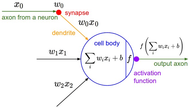
A biological inspiration#
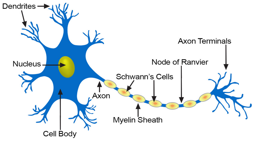
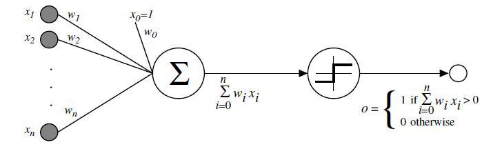
McCulloch & Pitts’ formal neuron (1943)#
Hebb’s rule (1949)#
Attempt to explain synaptic plasticity, the adaptation of brain neurons during the learning process.
“The general idea is an old one, that any two cells or systems of cells that are repeatedly active at the same time will tend to become ‘associated’ so that activity in one facilitates activity in the other.”
Franck Rosenblatt’s perceptron (1958)#
The perceptron learning algorithm#
Init randomly the \(\theta\) connection weights.
For each training sample \(x^{(i)}\):
Compute the perceptron output \(y'^{(i)}\)
Adjust weights : \(\theta_{next} = \theta + \eta (y^{(i)} - y'^{(i)}) x^{(i)}\)
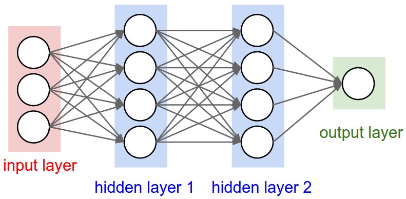
The MultiLayer Perceptron (MLP)#
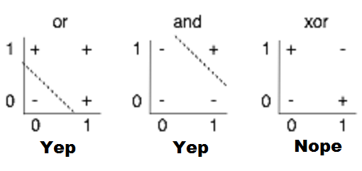
Minsky’s critic (1969)#
One perceptron cannot learn non-linearly separable functions.
At the time, no learning algorithm existed for training the hidden layers of a MLP.
Decisive breakthroughs (1970s-1990s)#
1974: backpropagation theory (P. Werbos).
1986: learning through backpropagation (Rumelhart, Hinton, Williams).
1991: universal approximation theorem (Hornik, Stinchcombe, White).
1989: first researchs on deep neural nets (LeCun, Bengio).
Neural networks fundamentals#
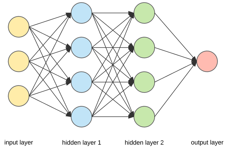
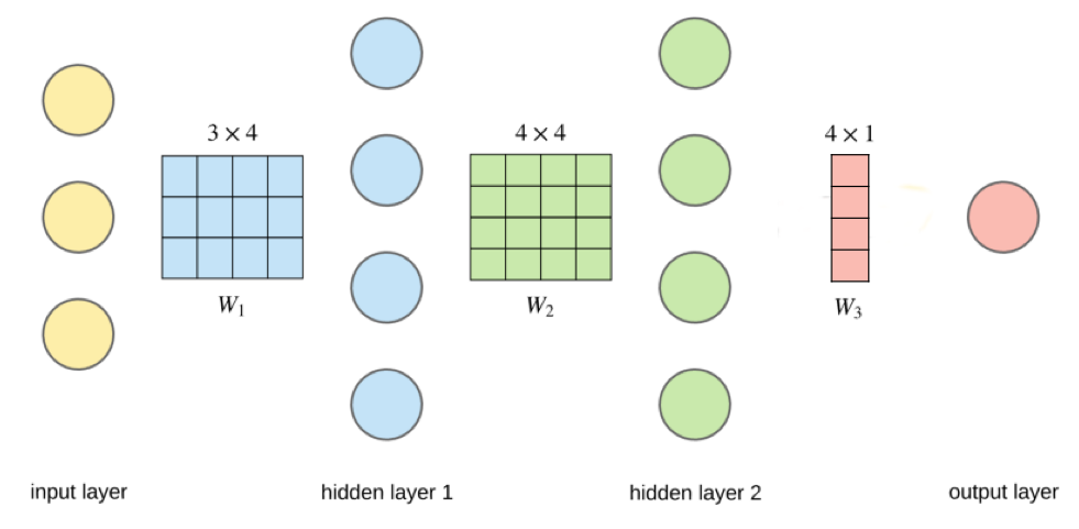
Anatomy of a network#
Neuron output#
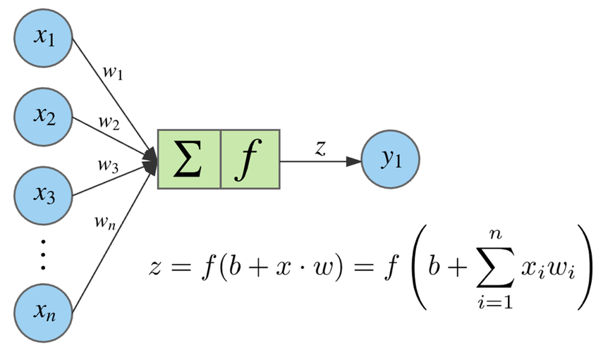
Activation functions#
Applied to the weighted sum of neuron inputs to produce its output.
Always non-linear. If not, the whole network could only apply a linear transformation to its inputs and couldn’t solve complex problems.
The main ones are:
sigmoid (logistic function)
tanh (hyberbolic tangent)
ReLU (Rectified Linear Unit)
See Activation functions for details.
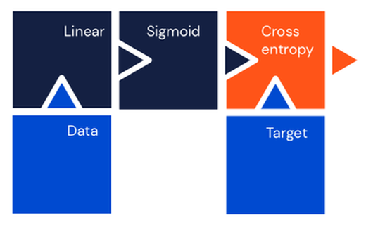
Single neuron classifier#
Equivalent to logistic regression.
Single layer multiclass classifier#
Equivalent to softmax regression.
Universal approximation theorem (1991)#
The hidden layers of a neural network transform their input space.
A network can be seen as a series of non-linear compositions applied to the input data.
Given appropriate complexity and appropriate learning, a network can theorically approximate any continuous function.
One of the most important theoretical results for neural networks.
Training neural networks#
Training and inference#
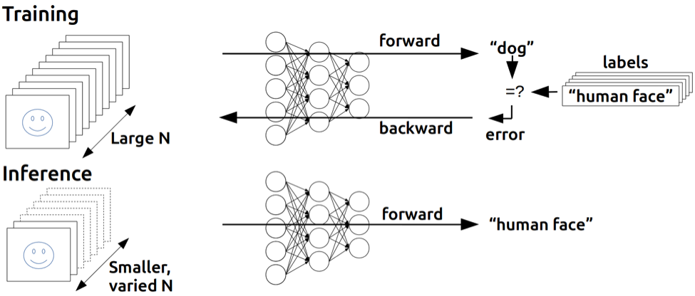
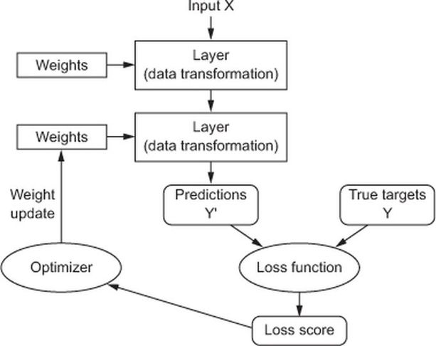
Learning algorithm#
Weights initialization#
To facilitate training, initial weights must be:
non-zero
random
have small values
Several techniques exist. A commonly used one is Xavier initialization.
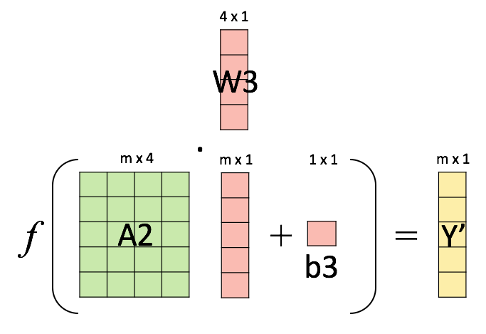
Vectorization of computations#
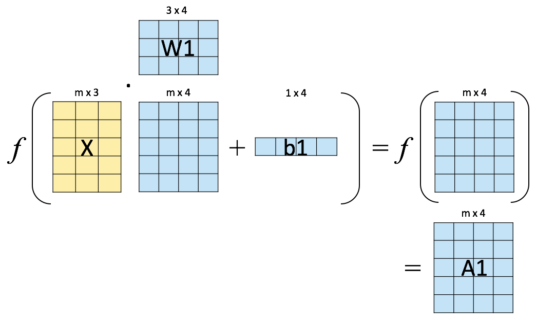
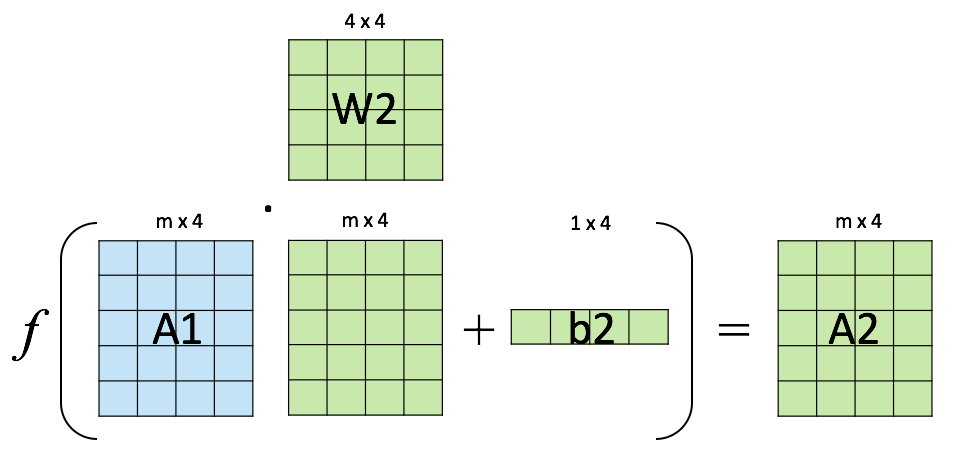
Output layer result#
Weights update#
Objective: minimize the loss function that computes the distance between expected and actual results.
Method : gradient descent.
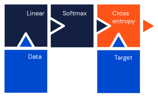
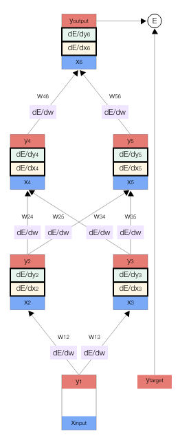
Neural networks as computational graphs#
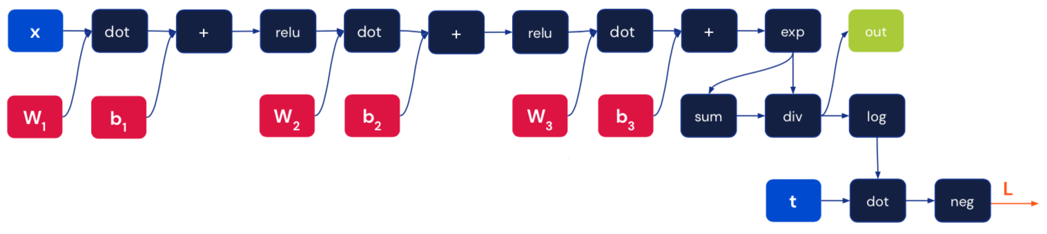
Backpropagation#
Objective: compute \(\nabla_{\boldsymbol{\theta}}\mathcal{L}(\boldsymbol{\theta})\), the loss function gradient w.r.t. all the network weights.
Method: apply the chain rule to compute partial derivatives backwards, starting from the current output.
Visual demo of backpropagation#
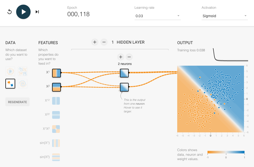
Interactive recap#
Neural networks in action#
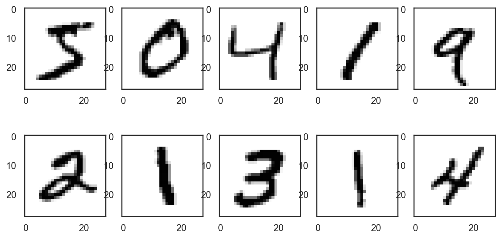
Example: training a multiclass classifier to recognize handwritten digits#
The MNIST digits dataset contains 70,000 handwritten digits, stored as 28x28 grayscale images.
Once challenging for ML model, it’s now the “Hello World” of Computer Vision.
# Load the Keras MNIST digits dataset
(train_images, train_labels), (test_images, test_labels) = mnist.load_data()

print(f"Training images: {train_images.shape}. Training labels: {train_labels.shape}")
print(f"Test images: {test_images.shape}. Test labels: {test_labels.shape}")
Training images: (60000, 28, 28). Training labels: (60000,)
Test images: (10000, 28, 28). Test labels: (10000,)
# Plot the first 10 digits
with sns.axes_style("white"):  # Temporary hide Seaborn grid lines
    plt.figure(figsize=(10, 5))
    for i in range(10):
        digit = train_images[i]
        fig = plt.subplot(2, 5, i + 1)
        plt.imshow(digit, cmap=plt.cm.binary)
# Labels are integer scalars between 0 and 9
df_train_labels = pd.DataFrame(train_labels)
df_train_labels.columns = {"digit"}
df_train_labels.sample(n=8)
| digit | |
|---|---|
| 22922 | 2 |
| 52071 | 7 |
| 56722 | 7 |
| 59578 | 6 |
| 3130 | 1 |
| 13430 | 4 |
| 57796 | 9 |
| 10892 | 1 |
Data preprocessing#
# Change pixel values from (0, 255) to (0, 1)
x_train = train_images.astype("float32") / 255
x_test = test_images.astype("float32") / 255
# One-hot encoding of expected results
y_train = to_categorical(train_labels)
y_test = to_categorical(test_labels)

print(f"y_train: {y_train.shape}")
print(f"y_test: {y_test.shape}")

# Show a sample of encoded input
df_y_train = pd.DataFrame(y_train)
df_y_train.sample(n=8)
y_train: (60000, 10)
y_test: (10000, 10)
| 0 | 1 | 2 | 3 | 4 | 5 | 6 | 7 | 8 | 9 | |
|---|---|---|---|---|---|---|---|---|---|---|
| 37645 | 0.0 | 0.0 | 0.0 | 0.0 | 1.0 | 0.0 | 0.0 | 0.0 | 0.0 | 0.0 |
| 57708 | 0.0 | 0.0 | 0.0 | 0.0 | 1.0 | 0.0 | 0.0 | 0.0 | 0.0 | 0.0 |
| 17103 | 0.0 | 0.0 | 0.0 | 1.0 | 0.0 | 0.0 | 0.0 | 0.0 | 0.0 | 0.0 |
| 53787 | 0.0 | 1.0 | 0.0 | 0.0 | 0.0 | 0.0 | 0.0 | 0.0 | 0.0 | 0.0 |
| 51129 | 0.0 | 1.0 | 0.0 | 0.0 | 0.0 | 0.0 | 0.0 | 0.0 | 0.0 | 0.0 |
| 10122 | 0.0 | 0.0 | 1.0 | 0.0 | 0.0 | 0.0 | 0.0 | 0.0 | 0.0 | 0.0 |
| 6214 | 0.0 | 0.0 | 0.0 | 0.0 | 0.0 | 0.0 | 0.0 | 0.0 | 1.0 | 0.0 |
| 38880 | 0.0 | 0.0 | 0.0 | 0.0 | 0.0 | 0.0 | 0.0 | 0.0 | 0.0 | 1.0 |
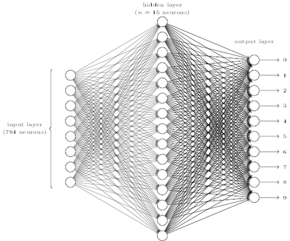
Network architecture for MNIST#
# Create the nn model
model = Sequential()
# The 28x28 images are flattened into a vector of 28*28 elements
model.add(Flatten(input_shape=(28, 28)))
model.add(Dense(15, activation="relu"))
# The softmax function creates a probability distribution
model.add(Dense(10, activation="softmax"))

# Describe the model
model.summary()
Metal device set to: Apple M1 Pro
Model: "sequential"
_________________________________________________________________
 Layer (type)                Output Shape              Param #
=================================================================
 flatten (Flatten)           (None, 784)               0

 dense (Dense)               (None, 15)                11775

 dense_1 (Dense)             (None, 10)                160

=================================================================
Total params: 11,935
Trainable params: 11,935
Non-trainable params: 0
_________________________________________________________________
# Train the model and show results
model.compile(
optimizer="rmsprop", loss="categorical_crossentropy", metrics=["accuracy"]
)
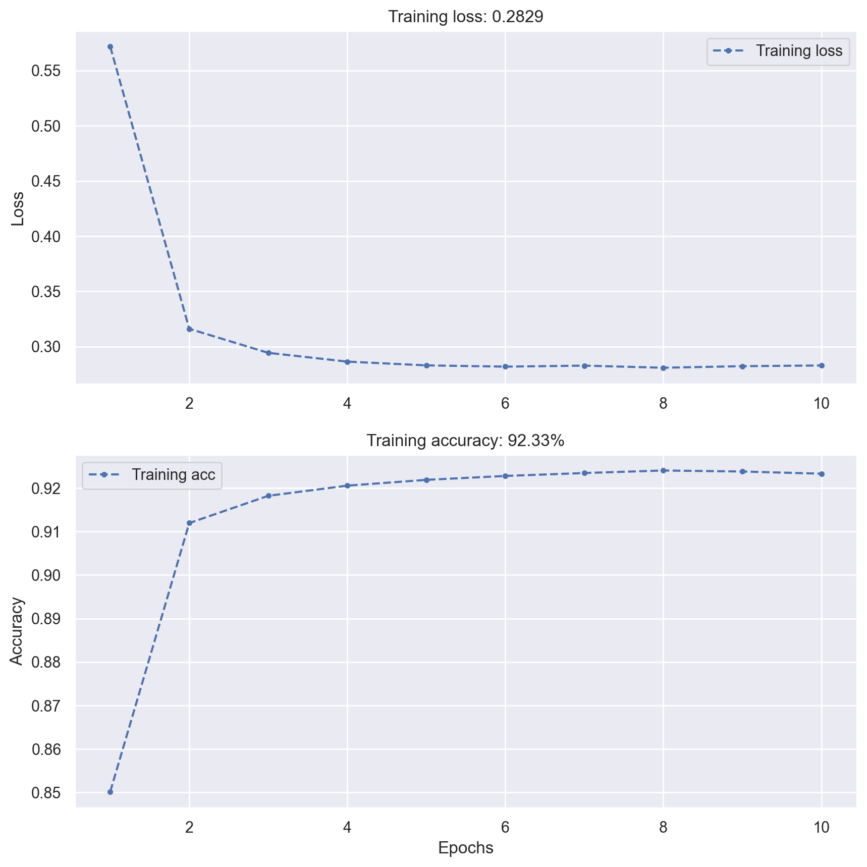
history = model.fit(x_train, y_train, verbose=0, epochs=10, batch_size=128)
plot_loss_acc(history)
2023-05-25 18:59:24.489324: W tensorflow/tsl/platform/profile_utils/cpu_utils.cc:128] Failed to get CPU frequency: 0 Hz
# Evaluate the model on test data
_, test_acc = model.evaluate(x_test, y_test, verbose=0)

print(f"Test accuracy: {test_acc:.5f}")
Test accuracy: 0.92060
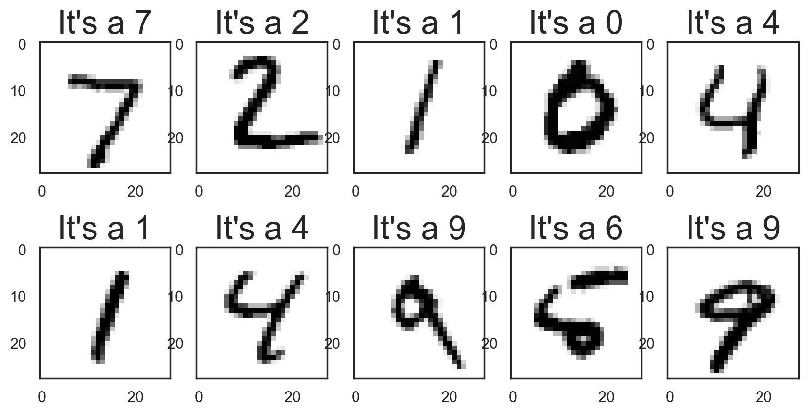
# Plot the first 10 test digits with associated predictions

# Temporary hide Seaborn grid lines
with sns.axes_style("white"):
    plt.figure(figsize=(10, 5))
    for i in range(10):
        digit = test_images[i]
        prediction = np.argmax(model.predict(digit.reshape((1, 28, 28))))
        fig = plt.subplot(2, 5, i + 1)
        plt.title("It's a {:d}".format(prediction), fontsize=24)
        plt.imshow(digit, cmap=plt.cm.binary)
1/1 [==============================] - 0s 345ms/step
1/1 [==============================] - 0s 11ms/step
1/1 [==============================] - 0s 11ms/step
1/1 [==============================] - 0s 11ms/step
1/1 [==============================] - 0s 11ms/step
1/1 [==============================] - 0s 11ms/step
1/1 [==============================] - 0s 11ms/step
1/1 [==============================] - 0s 11ms/step
1/1 [==============================] - 0s 11ms/step
1/1 [==============================] - 0s 11ms/step
# Saving model for future use
model_json = model.to_json()

with open("model.json", "w") as json_file:
    json_file.write(model_json)

model.save_weights("model.h5")
Tuning neural networks#
Hyperparameters choice#
Number of layers
Number of neurons on hidden layers
Activation functions
Learning rate
Mini-batch size
…
The optimization/generalization dilemna#
Tackle underfitting:
Use a more complex network
Train the network longer
Tackle overfitting:
Use more training data
Limit the network size
Introduce regularization
Introduce dropout
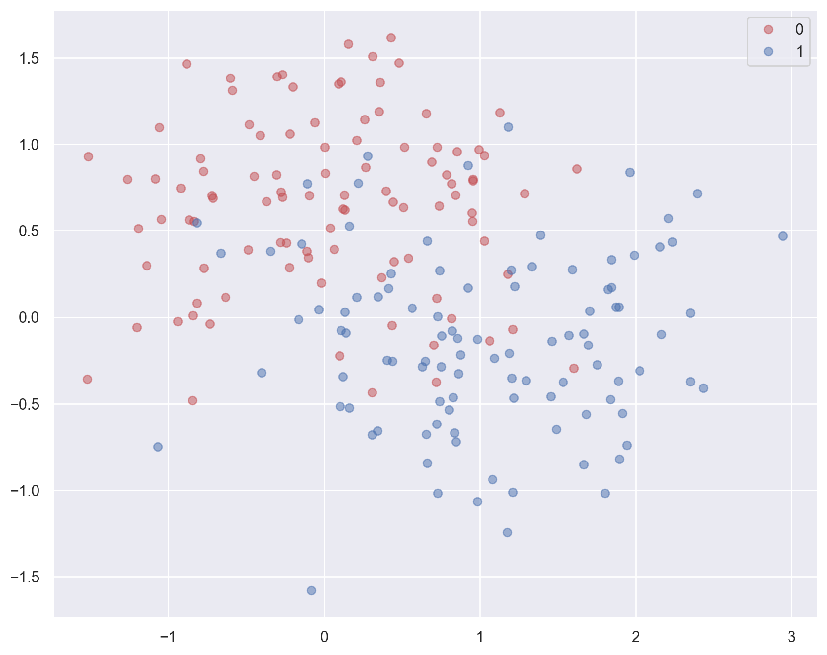
Observing underfitting and overfitting#
(Inspired by the article Implementing a Neural Network from Scratch)
# Generate moon-shaped data with some noise
x_train, y_train = make_moons(200, noise=0.40)

plot_planar_data(x_train, y_train)
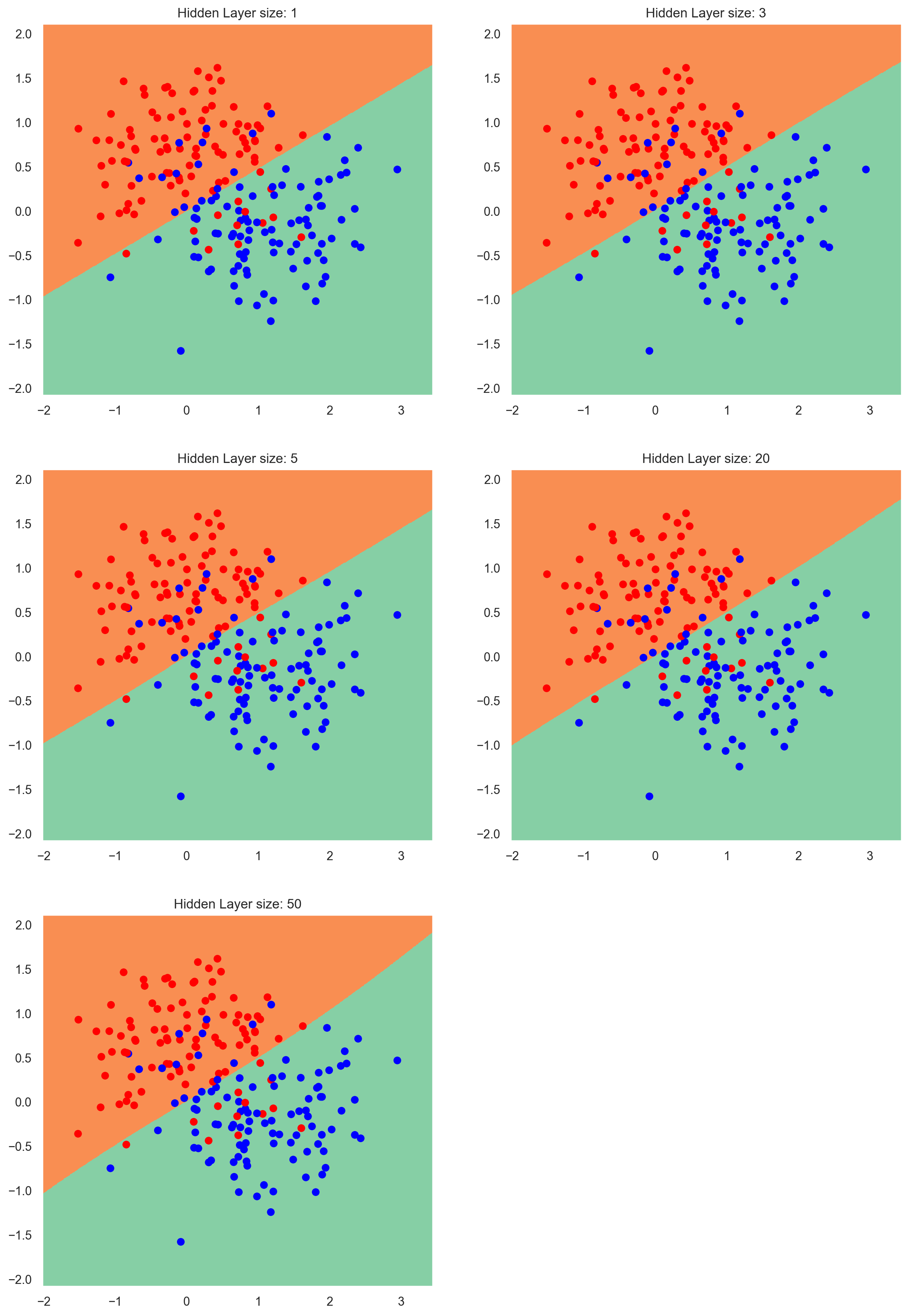
# Varying the hidden layer size to observe underfitting and overfitting

plt.figure(figsize=(14, 28))
hidden_layer_dimensions = [1, 3, 5, 20, 50]
for i, hidden_layer_size in enumerate(hidden_layer_dimensions):
    fig = plt.subplot(4, 2, i + 1)
    plt.title("Hidden Layer size: {:d}".format(hidden_layer_size))

    model = Sequential()
    model.add(Dense(hidden_layer_size, activation="tanh", input_shape=(2,)))
    model.add(Dense(1, activation="sigmoid"))
    model.compile(
        optimizer=SGD(lr=1.0), loss="binary_crossentropy", metrics=["accuracy"]
    )

    # Batch size = dataset size => batch gradient descent
    history = model.fit(
        x_train, y_train, verbose=0, epochs=5000, batch_size=x_train.shape[0]
    )

    plot_decision_boundary(lambda x: model.predict(x) > 0.5, x_train, y_train, fig)
WARNING:absl:At this time, the v2.11+ optimizer `tf.keras.optimizers.SGD` runs slowly on M1/M2 Macs, please use the legacy Keras optimizer instead, located at `tf.keras.optimizers.legacy.SGD`.
WARNING:absl:`lr` is deprecated in Keras optimizer, please use `learning_rate` or use the legacy optimizer, e.g.,tf.keras.optimizers.legacy.SGD.
WARNING:absl:There is a known slowdown when using v2.11+ Keras optimizers on M1/M2 Macs. Falling back to the legacy Keras optimizer, i.e., `tf.keras.optimizers.legacy.SGD`.
7180/7180 [==============================] - 9s 1ms/step
WARNING:absl:At this time, the v2.11+ optimizer `tf.keras.optimizers.SGD` runs slowly on M1/M2 Macs, please use the legacy Keras optimizer instead, located at `tf.keras.optimizers.legacy.SGD`.
WARNING:absl:`lr` is deprecated in Keras optimizer, please use `learning_rate` or use the legacy optimizer, e.g.,tf.keras.optimizers.legacy.SGD.
WARNING:absl:There is a known slowdown when using v2.11+ Keras optimizers on M1/M2 Macs. Falling back to the legacy Keras optimizer, i.e., `tf.keras.optimizers.legacy.SGD`.
7180/7180 [==============================] - 10s 1ms/step
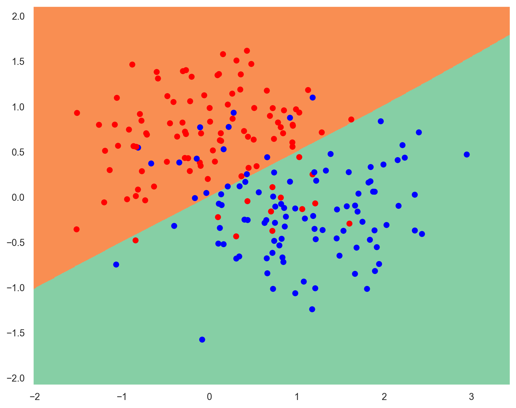
Tackling overfitting#
Regularization#
Limit weights values by adding a penalty to the loss function.
\(\lambda\) is called the regularization rate.
model = Sequential()

# Use L1 regularization on hidden layer
model.add(
    Dense(
        50,
        activation="tanh",
        input_shape=(2,),
        kernel_regularizer=regularizers.l1(0.001),
    )
)
model.add(Dense(1, activation="sigmoid"))
model.compile(optimizer=SGD(lr=1.0), loss="binary_crossentropy", metrics=["accuracy"])

# Batch size = dataset size => batch gradient descent
history = model.fit(
    x_train, y_train, verbose=0, epochs=5000, batch_size=x_train.shape[0]
)

plot_decision_boundary(lambda x: model.predict(x) > 0.5, x_train, y_train)
WARNING:absl:At this time, the v2.11+ optimizer `tf.keras.optimizers.SGD` runs slowly on M1/M2 Macs, please use the legacy Keras optimizer instead, located at `tf.keras.optimizers.legacy.SGD`.
WARNING:absl:`lr` is deprecated in Keras optimizer, please use `learning_rate` or use the legacy optimizer, e.g.,tf.keras.optimizers.legacy.SGD.
WARNING:absl:There is a known slowdown when using v2.11+ Keras optimizers on M1/M2 Macs. Falling back to the legacy Keras optimizer, i.e., `tf.keras.optimizers.legacy.SGD`.
7180/7180 [==============================] - 10s 1ms/step
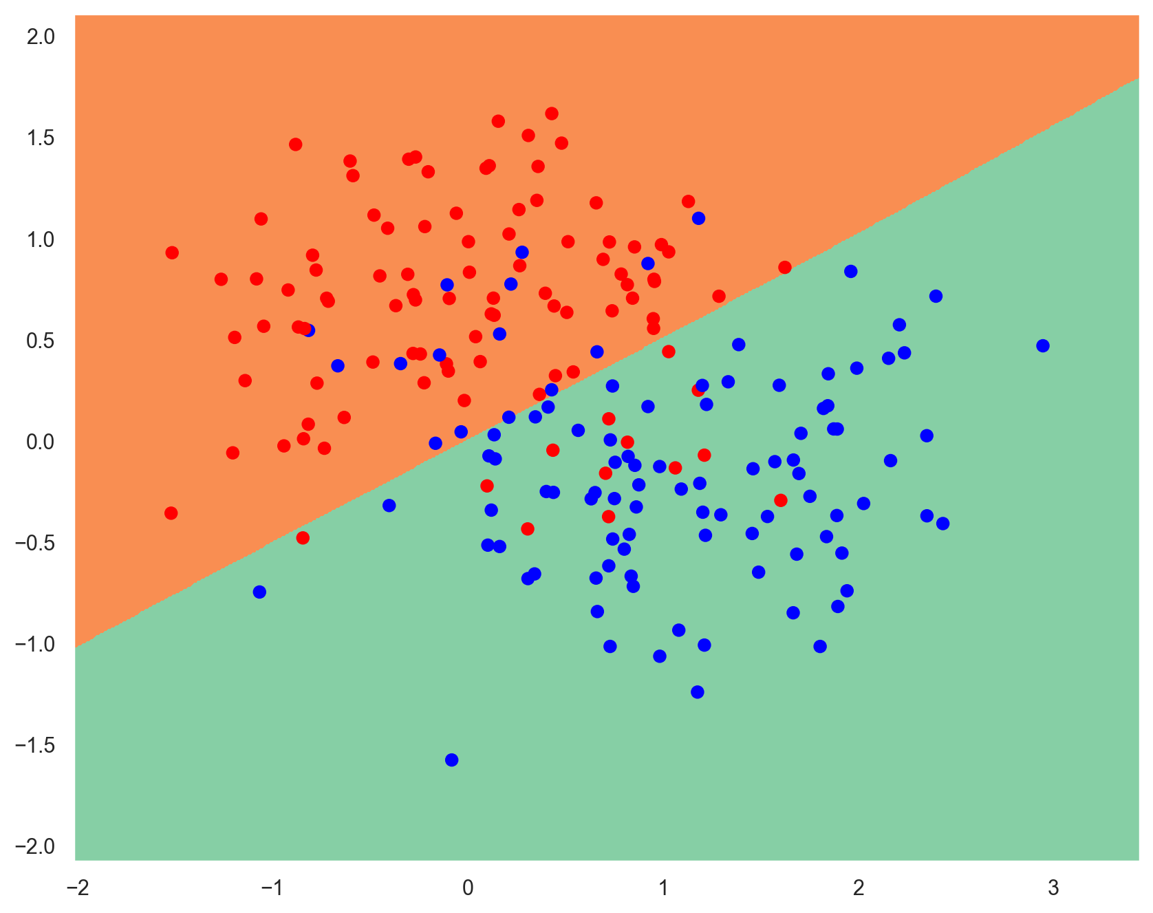
Dropout#
During training, some input units are randomly set to 0. The network must adapt and become more generic. The more units dropped out, the stronger the regularization.
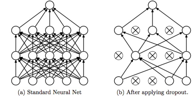
model = Sequential()

model.add(Dense(50, activation="tanh", input_shape=(2,)))
# Applies 25% dropout on previous layer
model.add(Dropout(0.25))
model.add(Dense(1, activation="sigmoid"))
model.compile(optimizer=SGD(lr=1.0), loss="binary_crossentropy", metrics=["accuracy"])

# Batch size = dataset size => batch gradient descent
history = model.fit(
    x_train, y_train, verbose=0, epochs=5000, batch_size=x_train.shape[0]
)

plot_decision_boundary(lambda x: model.predict(x) > 0.5, x_train, y_train)
WARNING:absl:At this time, the v2.11+ optimizer `tf.keras.optimizers.SGD` runs slowly on M1/M2 Macs, please use the legacy Keras optimizer instead, located at `tf.keras.optimizers.legacy.SGD`.
WARNING:absl:`lr` is deprecated in Keras optimizer, please use `learning_rate` or use the legacy optimizer, e.g.,tf.keras.optimizers.legacy.SGD.
WARNING:absl:There is a known slowdown when using v2.11+ Keras optimizers on M1/M2 Macs. Falling back to the legacy Keras optimizer, i.e., `tf.keras.optimizers.legacy.SGD`.
7180/7180 [==============================] - 11s 1ms/step
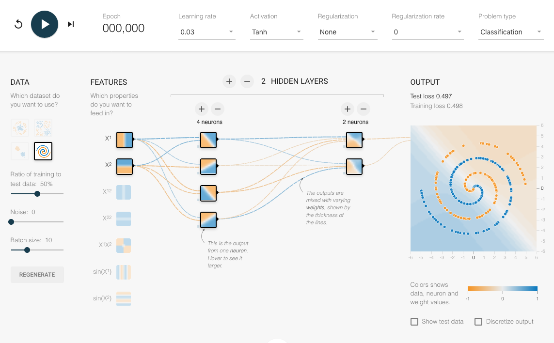
Interactive recap#
Overfitting on a real-world example#
(Heavily inspired by a use case in François Chollet’s book Deep Learning With Python)
# Load the Keras IMDB dataset
# We only keep the top 10,000 most frequently occuring words in the training data
(train_data, train_labels), (test_data, test_labels) = imdb.load_data(num_words=10000)

print(f"Training data: {train_data.shape}. Training labels: {train_labels.shape}")

# Reviews are encoded as lists of word indexes
# Words are indexed by overall frequency in the dataset
print(f"First review: {train_data[0]}")

# Labels are binary integers: 0 for a negative review, 1 for a positive one
print(f"First label: {train_labels[0]}")
Downloading data from https://storage.googleapis.com/tensorflow/tf-keras-datasets/imdb.npz
17464789/17464789 [==============================] - 1s 0us/step
Training data: (25000,). Training labels: (25000,)
First review: [1, 14, 22, 16, 43, 530, 973, 1622, 1385, 65, 458, 4468, 66, 3941, 4, 173, 36, 256, 5, 25, 100, 43, 838, 112, 50, 670, 2, 9, 35, 480, 284, 5, 150, 4, 172, 112, 167, 2, 336, 385, 39, 4, 172, 4536, 1111, 17, 546, 38, 13, 447, 4, 192, 50, 16, 6, 147, 2025, 19, 14, 22, 4, 1920, 4613, 469, 4, 22, 71, 87, 12, 16, 43, 530, 38, 76, 15, 13, 1247, 4, 22, 17, 515, 17, 12, 16, 626, 18, 2, 5, 62, 386, 12, 8, 316, 8, 106, 5, 4, 2223, 5244, 16, 480, 66, 3785, 33, 4, 130, 12, 16, 38, 619, 5, 25, 124, 51, 36, 135, 48, 25, 1415, 33, 6, 22, 12, 215, 28, 77, 52, 5, 14, 407, 16, 82, 2, 8, 4, 107, 117, 5952, 15, 256, 4, 2, 7, 3766, 5, 723, 36, 71, 43, 530, 476, 26, 400, 317, 46, 7, 4, 2, 1029, 13, 104, 88, 4, 381, 15, 297, 98, 32, 2071, 56, 26, 141, 6, 194, 7486, 18, 4, 226, 22, 21, 134, 476, 26, 480, 5, 144, 30, 5535, 18, 51, 36, 28, 224, 92, 25, 104, 4, 226, 65, 16, 38, 1334, 88, 12, 16, 283, 5, 16, 4472, 113, 103, 32, 15, 16, 5345, 19, 178, 32]
First label: 1
# Show the first review as text

# word_index is a dictionary mapping words to an integer index
word_index = imdb.get_word_index()
# We reverse it, mapping integer indices to words
reverse_word_index = dict([(value, key) for (key, value) in word_index.items()])
# We decode the review; note that our indices were offset by 3
# because 0, 1 and 2 are reserved indices for "padding", "start of sequence", and "unknown".
decoded_review = " ".join([reverse_word_index.get(i - 3, "?") for i in train_data[0]])
print(decoded_review)
Downloading data from https://storage.googleapis.com/tensorflow/tf-keras-datasets/imdb_word_index.json
1641221/1641221 [==============================] - 0s 0us/step
? this film was just brilliant casting location scenery story direction everyone's really suited the part they played and you could just imagine being there robert ? is an amazing actor and now the same being director ? father came from the same scottish island as myself so i loved the fact there was a real connection with this film the witty remarks throughout the film were great it was just brilliant so much that i bought the film as soon as it was released for ? and would recommend it to everyone to watch and the fly fishing was amazing really cried at the end it was so sad and you know what they say if you cry at a film it must have been good and this definitely was also ? to the two little boy's that played the ? of norman and paul they were just brilliant children are often left out of the ? list i think because the stars that play them all grown up are such a big profile for the whole film but these children are amazing and should be praised for what they have done don't you think the whole story was so lovely because it was true and was someone's life after all that was shared with us all
# Preparation of data for training


def vectorize_sequences(sequences, dimension=10000):
    """One-hot encode a vector of sequences into a binary matrix (number of sequences, dimension)"""

    # Example : [[3, 5]] -> [[0. 0. 0. 1. 0. 1. 0...]]

    results = np.zeros((len(sequences), dimension))
    # set specific indices of results[i] to 1s
    for i, sequence in enumerate(sequences):
        results[i, sequence] = 1.0
    return results


# Turn reviews into vectors of 0s and 1s (one-hot encoding)
x_train = vectorize_sequences(train_data)
x_test = vectorize_sequences(test_data)

# Set apart the first 10,000 reviews as validation data
x_val, x_train = x_train[:10000], x_train[10000:]
y_val, y_train = train_labels[:10000], train_labels[10000:]

y_test = test_labels

print(f"x_train: {x_train.shape}. x_val: {x_val.shape}")
x_train: (15000, 10000). x_val: (10000, 10000)
# Show a sample of encoded input
df_x_train = pd.DataFrame(x_train)
df_x_train.sample(n=10)
| 0 | 1 | 2 | 3 | 4 | 5 | 6 | 7 | 8 | 9 | ... | 9990 | 9991 | 9992 | 9993 | 9994 | 9995 | 9996 | 9997 | 9998 | 9999 | |
|---|---|---|---|---|---|---|---|---|---|---|---|---|---|---|---|---|---|---|---|---|---|
| 5738 | 0.0 | 1.0 | 1.0 | 0.0 | 1.0 | 1.0 | 1.0 | 1.0 | 1.0 | 1.0 | ... | 0.0 | 0.0 | 0.0 | 0.0 | 0.0 | 0.0 | 0.0 | 0.0 | 0.0 | 0.0 |
| 2392 | 0.0 | 1.0 | 1.0 | 0.0 | 1.0 | 1.0 | 1.0 | 1.0 | 1.0 | 0.0 | ... | 0.0 | 0.0 | 0.0 | 0.0 | 0.0 | 0.0 | 0.0 | 0.0 | 0.0 | 0.0 |
| 3824 | 0.0 | 1.0 | 1.0 | 0.0 | 1.0 | 1.0 | 1.0 | 1.0 | 1.0 | 1.0 | ... | 0.0 | 0.0 | 0.0 | 0.0 | 0.0 | 0.0 | 0.0 | 0.0 | 0.0 | 0.0 |
| 4586 | 0.0 | 1.0 | 1.0 | 0.0 | 1.0 | 1.0 | 1.0 | 1.0 | 1.0 | 1.0 | ... | 0.0 | 0.0 | 0.0 | 0.0 | 0.0 | 0.0 | 0.0 | 0.0 | 0.0 | 0.0 |
| 12950 | 0.0 | 1.0 | 1.0 | 0.0 | 1.0 | 1.0 | 1.0 | 1.0 | 1.0 | 1.0 | ... | 0.0 | 0.0 | 0.0 | 0.0 | 0.0 | 0.0 | 0.0 | 0.0 | 0.0 | 0.0 |
| 11154 | 0.0 | 1.0 | 1.0 | 0.0 | 1.0 | 1.0 | 1.0 | 1.0 | 1.0 | 1.0 | ... | 0.0 | 0.0 | 0.0 | 0.0 | 0.0 | 0.0 | 0.0 | 0.0 | 0.0 | 0.0 |
| 186 | 0.0 | 1.0 | 1.0 | 0.0 | 1.0 | 1.0 | 1.0 | 1.0 | 1.0 | 1.0 | ... | 0.0 | 0.0 | 0.0 | 0.0 | 0.0 | 0.0 | 0.0 | 0.0 | 0.0 | 0.0 |
| 11459 | 0.0 | 1.0 | 1.0 | 0.0 | 1.0 | 1.0 | 1.0 | 1.0 | 1.0 | 1.0 | ... | 0.0 | 0.0 | 0.0 | 0.0 | 0.0 | 0.0 | 0.0 | 0.0 | 0.0 | 0.0 |
| 3254 | 0.0 | 1.0 | 1.0 | 0.0 | 1.0 | 1.0 | 1.0 | 1.0 | 1.0 | 1.0 | ... | 0.0 | 0.0 | 0.0 | 0.0 | 0.0 | 0.0 | 0.0 | 0.0 | 0.0 | 0.0 |
| 6775 | 0.0 | 1.0 | 1.0 | 0.0 | 1.0 | 1.0 | 1.0 | 1.0 | 1.0 | 0.0 | ... | 0.0 | 0.0 | 0.0 | 0.0 | 0.0 | 0.0 | 0.0 | 0.0 | 0.0 | 0.0 |
10 rows × 10000 columns
# Build a nn with two hidden layers to demonstrate overfitting
model = Sequential()
model.add(Dense(16, activation="relu", input_shape=(10000,)))
model.add(Dense(16, activation="relu"))
model.add(Dense(1, activation="sigmoid"))

# Show model info
model.summary()
Model: "sequential_8"
_________________________________________________________________
 Layer (type)                Output Shape              Param #
=================================================================
 dense_16 (Dense)            (None, 16)                160016

 dense_17 (Dense)            (None, 16)                272

 dense_18 (Dense)            (None, 1)                 17

=================================================================
Total params: 160,305
Trainable params: 160,305
Non-trainable params: 0
_________________________________________________________________
model.compile(optimizer="rmsprop", loss="binary_crossentropy", metrics=["accuracy"])

# We also record validation history during training
history = model.fit(
    x_train, y_train, epochs=20, verbose=0, batch_size=512, validation_data=(x_val, y_val)
)
plot_loss_acc(history)
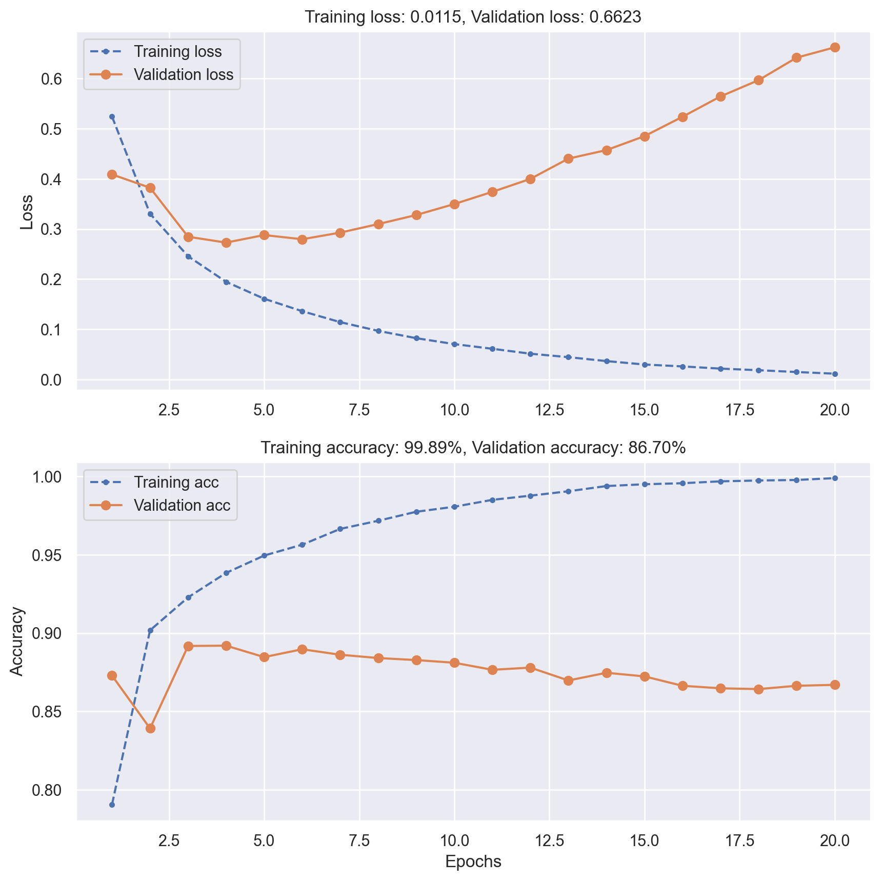
# Evaluate model performance on test data
_, test_acc = model.evaluate(x_test, y_test, verbose=0)

print(f"Test accuracy: {test_acc:.5f}")
Test accuracy: 0.85048
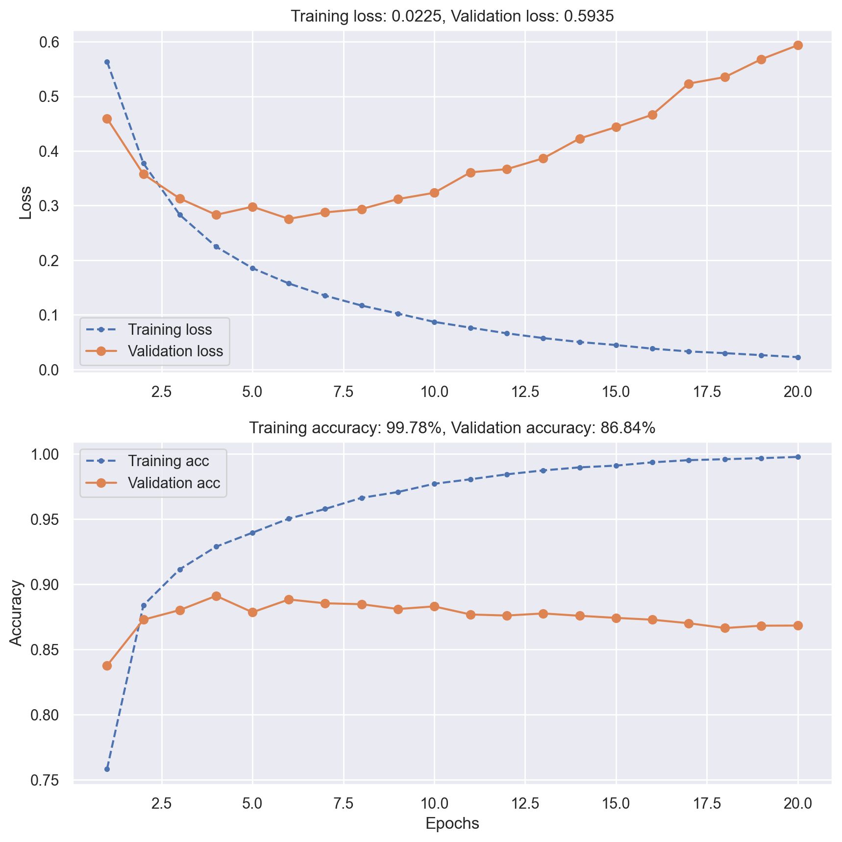
Reducing network size#
# Build and train a smaller network
model = Sequential()
model.add(Dense(8, activation="relu", input_shape=(10000,)))
model.add(Dense(8, activation="relu"))
model.add(Dense(1, activation="sigmoid"))

# Show model info to check the new number of parameters
model.summary()

model.compile(optimizer="rmsprop", loss="binary_crossentropy", metrics=["accuracy"])

history = model.fit(
    x_train, y_train, epochs=20, verbose=0, batch_size=512, validation_data=(x_val, y_val)
)
plot_loss_acc(history)
Model: "sequential_9"
_________________________________________________________________
 Layer (type)                Output Shape              Param #
=================================================================
 dense_19 (Dense)            (None, 8)                 80008

 dense_20 (Dense)            (None, 8)                 72

 dense_21 (Dense)            (None, 1)                 9

=================================================================
Total params: 80,089
Trainable params: 80,089
Non-trainable params: 0
_________________________________________________________________
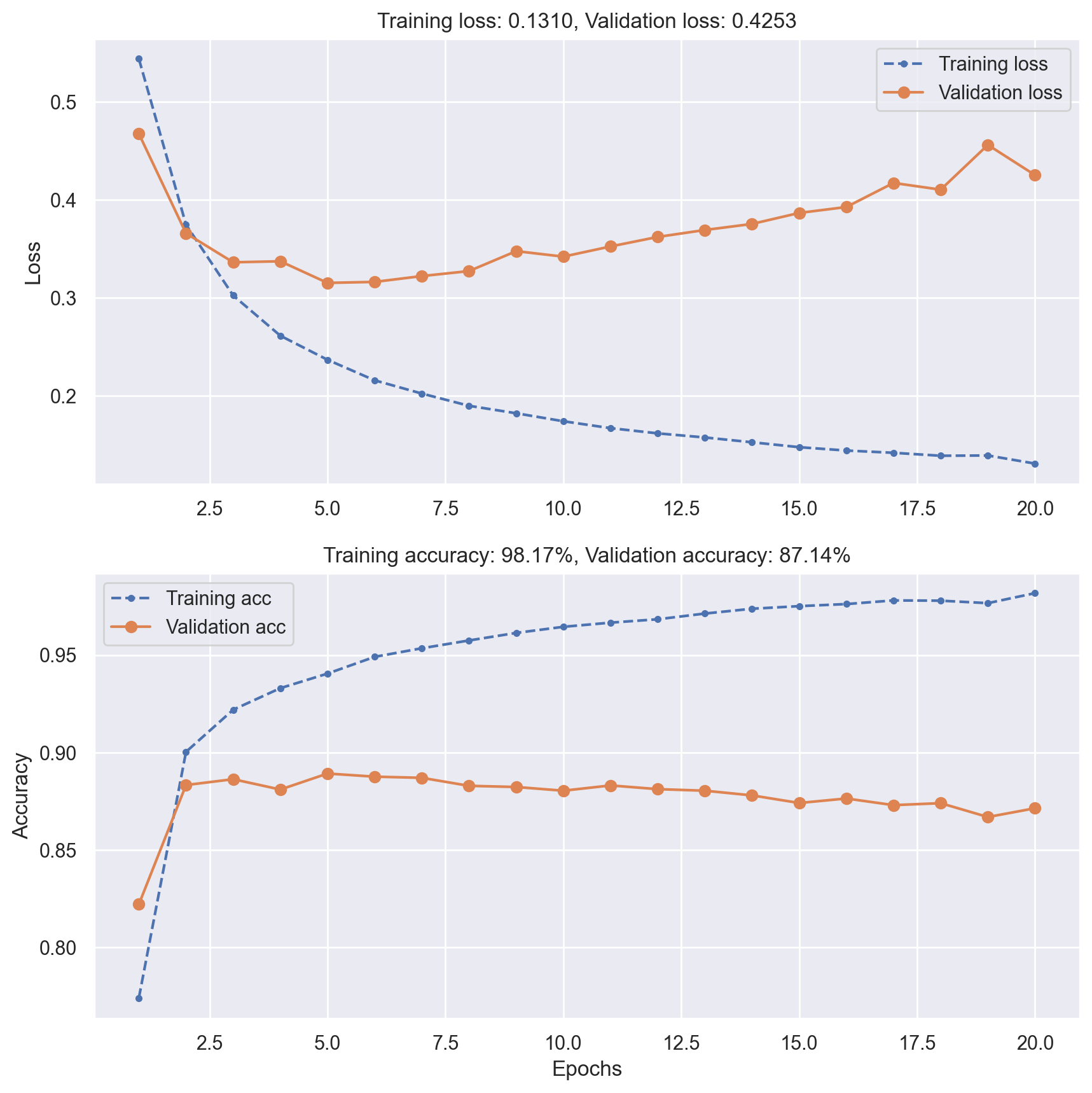
Regularization#
# Create the same model as before but now using L2 regularization
model = Sequential()
model.add(
    Dense(
        8,
        activation="relu",
        input_shape=(10000,),
        kernel_regularizer=regularizers.l2(0.001),
    )
)
model.add(Dense(8, activation="relu", kernel_regularizer=regularizers.l2(0.001)))
model.add(Dense(1, activation="sigmoid"))

# Show model info
model.summary()

model.compile(optimizer="rmsprop", loss="binary_crossentropy", metrics=["accuracy"])

history = model.fit(
    x_train, y_train, epochs=20, verbose=0, batch_size=512, validation_data=(x_val, y_val)
)
plot_loss_acc(history)
Model: "sequential_10"
_________________________________________________________________
 Layer (type)                Output Shape              Param #
=================================================================
 dense_22 (Dense)            (None, 8)                 80008

 dense_23 (Dense)            (None, 8)                 72

 dense_24 (Dense)            (None, 1)                 9

=================================================================
Total params: 80,089
Trainable params: 80,089
Non-trainable params: 0
_________________________________________________________________
Dropout#
# Add 50% dropout to the two hidden layers
model = Sequential()
model.add(
    Dense(
        8,
        activation="relu",
        input_shape=(10000,),
        kernel_regularizer=regularizers.l2(0.001),
    )
)
model.add(Dropout(0.5))
model.add(Dense(8, activation="relu", kernel_regularizer=regularizers.l2(0.001)))
model.add(Dropout(0.5))
model.add(Dense(1, activation="sigmoid"))

# Show model info
model.summary()

model.compile(optimizer="rmsprop", loss="binary_crossentropy", metrics=["accuracy"])

history = model.fit(
    x_train, y_train, epochs=20, verbose=0, batch_size=512, validation_data=(x_val, y_val)
)
plot_loss_acc(history)
Model: "sequential_11"
_________________________________________________________________
 Layer (type)                Output Shape              Param #
=================================================================
 dense_25 (Dense)            (None, 8)                 80008

 dropout_1 (Dropout)         (None, 8)                 0

 dense_26 (Dense)            (None, 8)                 72

 dropout_2 (Dropout)         (None, 8)                 0

 dense_27 (Dense)            (None, 1)                 9

=================================================================
Total params: 80,089
Trainable params: 80,089
Non-trainable params: 0
_________________________________________________________________
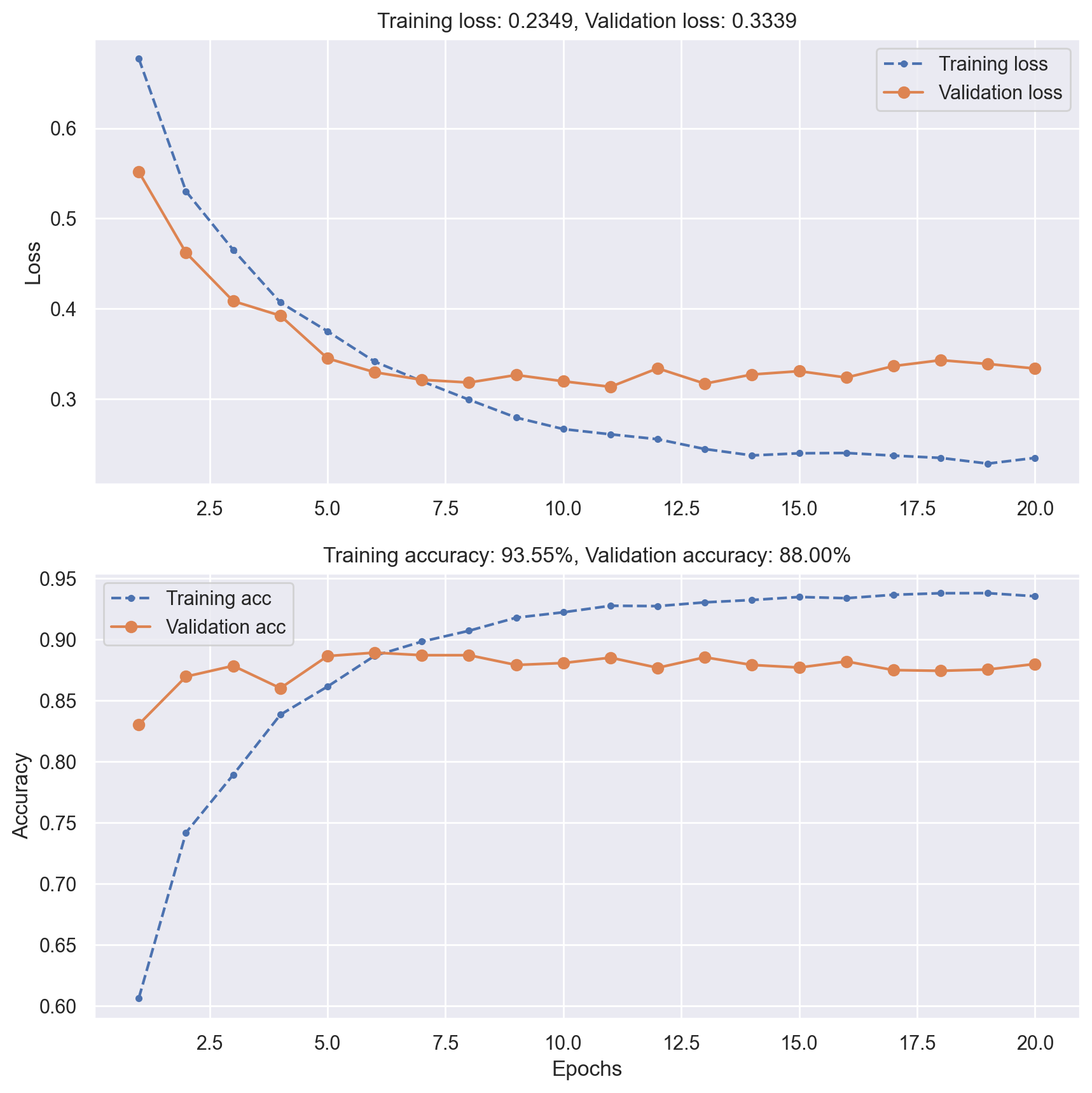
# Evaluate tuned model performance on test data
_, test_acc = model.evaluate(x_test, y_test, verbose=0)

print(f"Test accuracy: {test_acc:.5f}")
Test accuracy: 0.87024