Convolutional Neural Networks#
Environment setup#
import platform

print(f"Python version: {platform.python_version()}")

import numpy as np
import matplotlib.pyplot as plt
import seaborn as sns
import pandas as pd
Python version: 3.11.1
# Setup plots
%matplotlib inline
plt.rcParams["figure.figsize"] = 10, 8
%config InlineBackend.figure_format = 'retina'
sns.set()
import tensorflow as tf

print(f"TensorFlow version: {tf.__version__}")
print(f"Keras version: {tf.keras.__version__}")

# Device configuration
print("GPU found :)" if tf.config.list_physical_devices("GPU") else "No available GPU :/")

from tensorflow.keras.models import Sequential
from tensorflow.keras.layers import Dense, Flatten, Conv2D, MaxPooling2D, Dropout
from tensorflow.keras.datasets import fashion_mnist, cifar10
from tensorflow.keras.utils import to_categorical
from tensorflow.keras.applications import VGG16
TensorFlow version: 2.12.0
Keras version: 2.12.0
GPU found :)
Show code cell source
def plot_loss_acc(history):
    """Plot training and (optionally) validation loss and accuracy
    Takes a Keras History object as parameter"""

    loss = history.history["loss"]
    epochs = range(1, len(loss) + 1)

    plt.figure(figsize=(10, 10))

    plt.subplot(2, 1, 1)
    plt.plot(epochs, loss, ".--", label="Training loss")
    final_loss = loss[-1]
    title = "Training loss: {:.4f}".format(final_loss)
    plt.ylabel("Loss")
    if "val_loss" in history.history:
        val_loss = history.history["val_loss"]
        plt.plot(epochs, val_loss, "o-", label="Validation loss")
        final_val_loss = val_loss[-1]
        title += ", Validation loss: {:.4f}".format(final_val_loss)
    plt.title(title)
    plt.legend()

    acc = history.history["accuracy"]

    plt.subplot(2, 1, 2)
    plt.plot(epochs, acc, ".--", label="Training acc")
    final_acc = acc[-1]
    title = "Training accuracy: {:.2f}%".format(final_acc * 100)
    plt.xlabel("Epochs")
    plt.ylabel("Accuracy")
    if "val_accuracy" in history.history:
        val_acc = history.history["val_accuracy"]
        plt.plot(epochs, val_acc, "o-", label="Validation acc")
        final_val_acc = val_acc[-1]
        title += ", Validation accuracy: {:.2f}%".format(final_val_acc * 100)
    plt.title(title)
    plt.legend()
Architecture#
Justification#
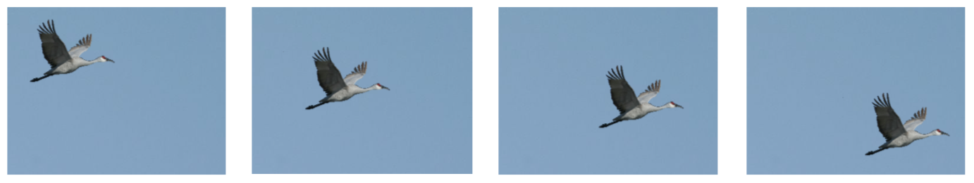
The visual world has the following properties:
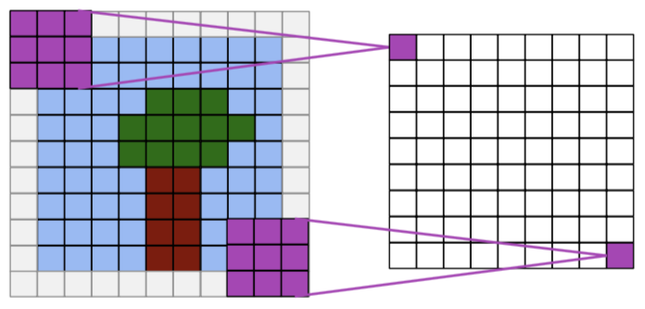
Translation invariance.
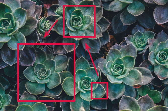
Locality: nearby pixels are more strongly correlated
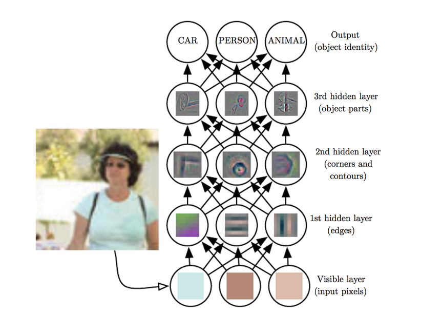
Spatial hierarchy: complex and abstract concepts are composed from simple, local elements.
Classical models are not designed to detect local patterns in images.
Topological structure of objects#

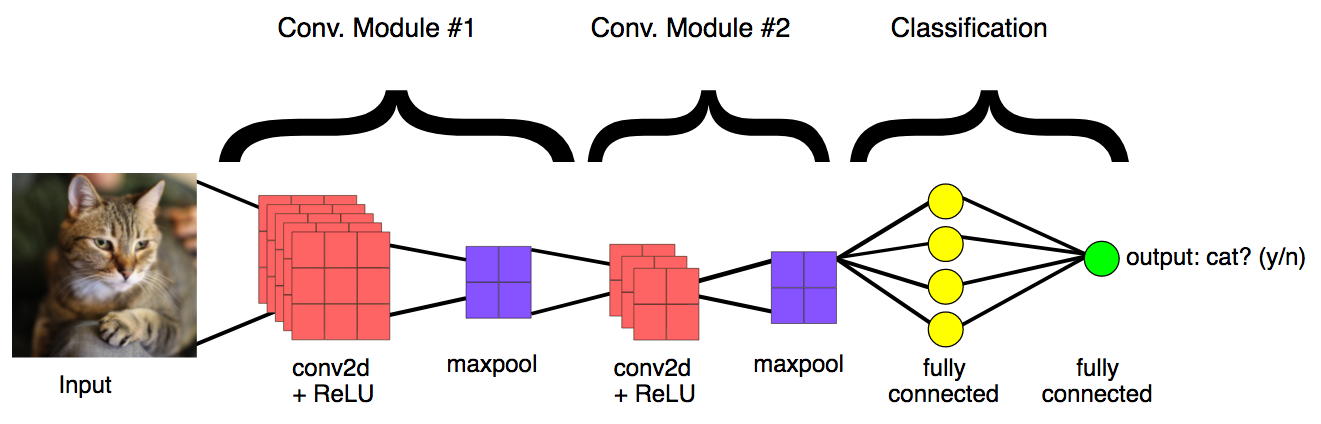
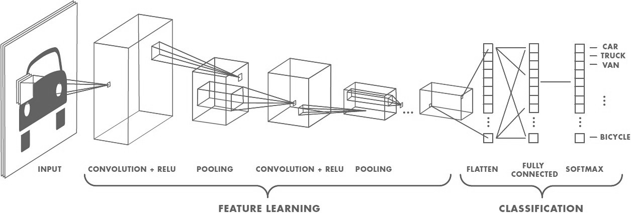
General CNN design#
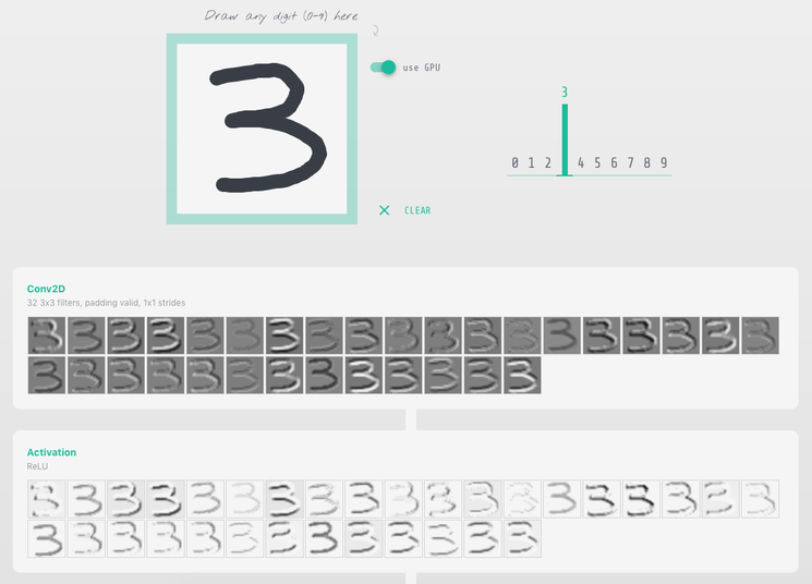
The convolution operation#
Apply a kernel to data. Result is called a feature map.
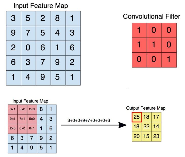
Convolution parameters#
Filter dimensions: 2D for images.
Filter size: generally 3x3 or 5x5.
Number of filters: determine the number of feature maps created by the convolution operation.
Stride: step for sliding the convolution window. Generally equal to 1.
Padding: blank rows/columns with all-zero values added on sides of the input feature map.
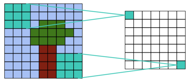
Preserving output dimensions with padding#
Valid padding#
Output size = input size - kernel size + 1
Full padding#
Output size = input size + kernel size - 1
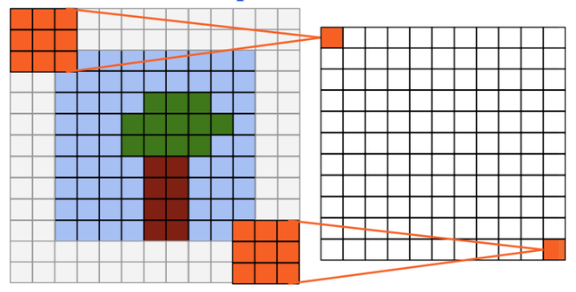
Same padding#
Output size = input size
Convolutions inputs and outputs: tensors#
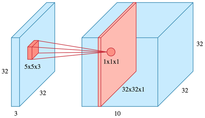
2D convolutions on 3D tensors#
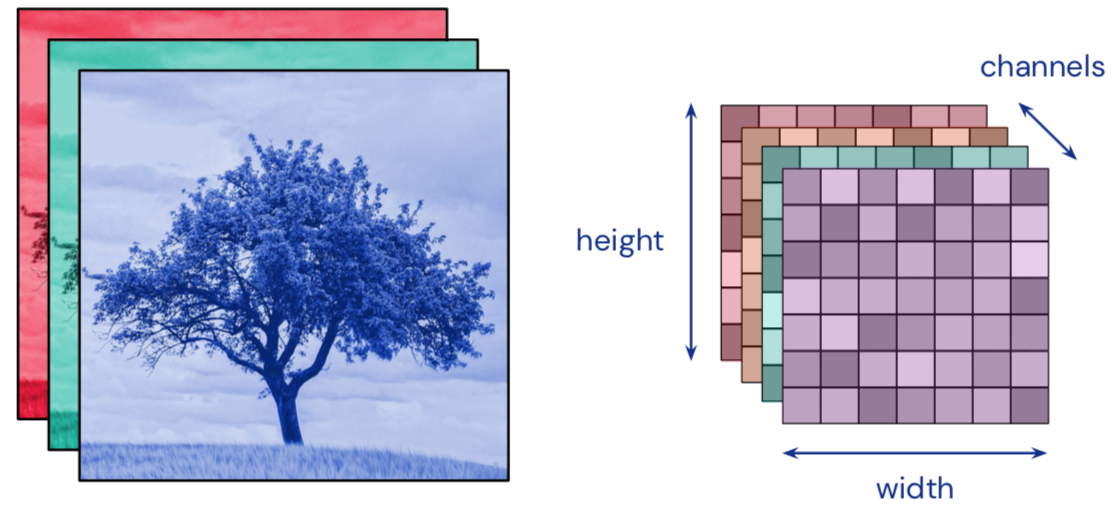
Convolution input data is 3-dimensional: images with height, width and color channels, or features maps produced by previous layers.
Each convolution filter is a collection of kernels with distinct weights, one for every input channel.
At each location, every input channel is convolved with the corresponding kernel. The results are summed to compute the (scalar) filter output for the location.
Sliding one filter over the input data produces a 2D output feature map.
Activation function#
Applied to the (scalar) convolution result.
Introduces non-linearity in the model.
Standard choice: \(ReLU(z) = max(0,z)\)
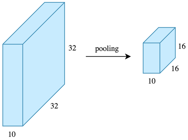
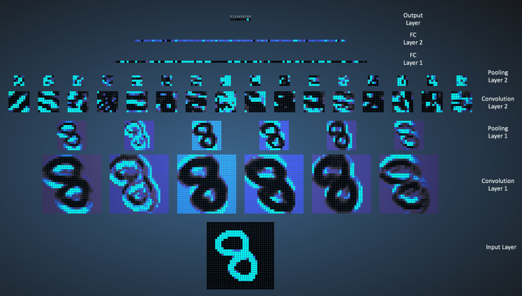
The pooling operation#
Reduces the dimensionality of feature maps.
Often done by selecting maximum values (max pooling).
Pooling result#
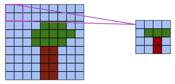
Pooling output#
Interpretation#
Convolution layers act as feature extractors.
Dense layers use the extracted features to classify data.
History#
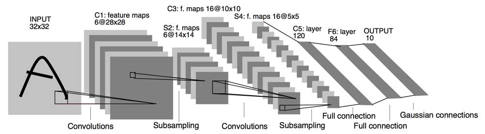
Humble beginnings: LeNet5 (1988)#
Show code cell source
from IPython.display import YouTubeVideo

YouTubeVideo("FwFduRA_L6Q")
The breakthrough: ILSVRC#
Worldwide image classification challenge based on the ImageNet dataset.
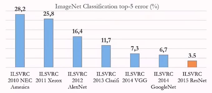
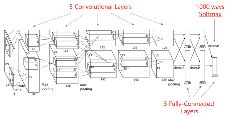
AlexNet (2012)#
Trained on 2 GPU for 5 to 6 days.
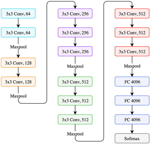
VGG (2014)#
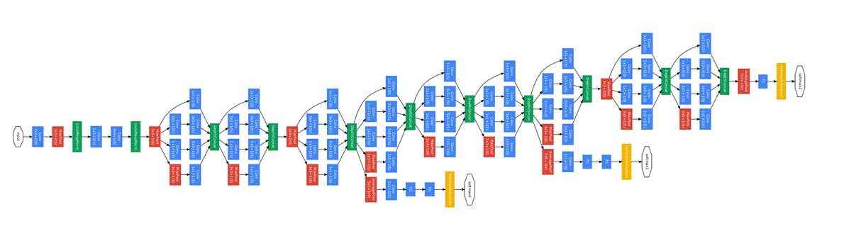
GoogLeNet/Inception (2014)#
9 Inception modules, more than 100 layers.
Trained on several GPU for about a week.
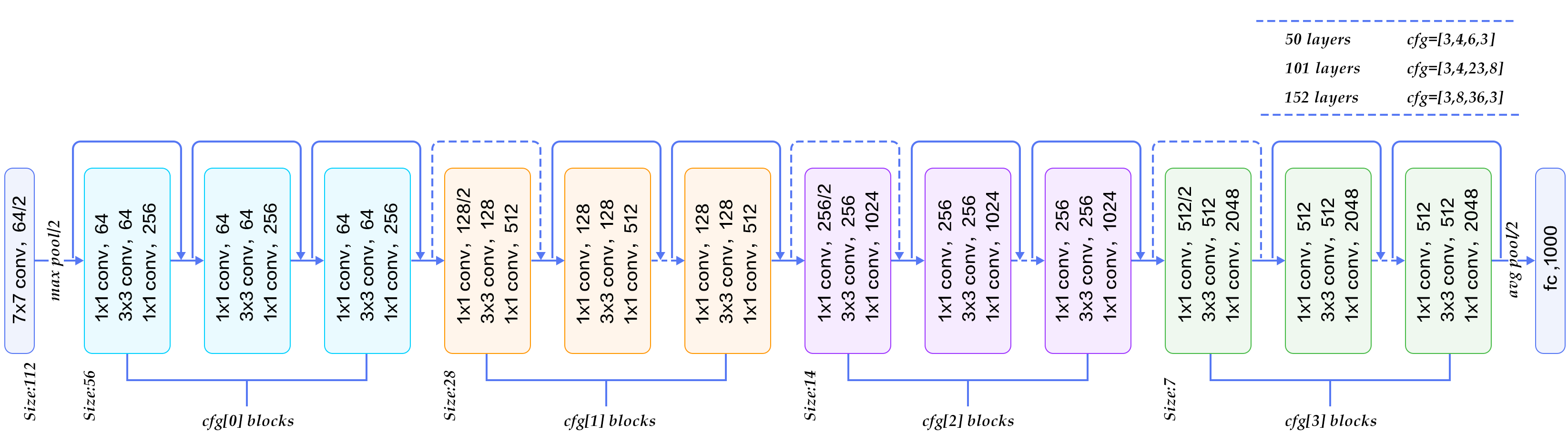
Microsoft ResNet (2015)#
152 layers, trained on 8 GPU for 2 to 3 weeks.
Smaller error rate than a average human.

Depth: challenges and solutions#
Challenges
Computational complexity
Optimization difficulties
Solutions
Careful initialization
Sophisticated optimizers
Normalisation layers
Network design
Training a convnet#
General principle#
Same principle as a dense neural network: backpropagation + gradient descent.
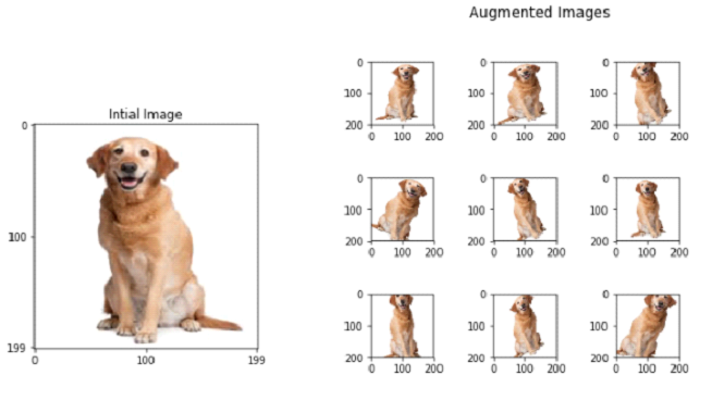
Data augmentation#
By design, convnets are only robust against translation. Data augmentation can make them robust against rotation and scaling.
Principle: the dataset is enriched with new samples created by applying operations on existing ones.
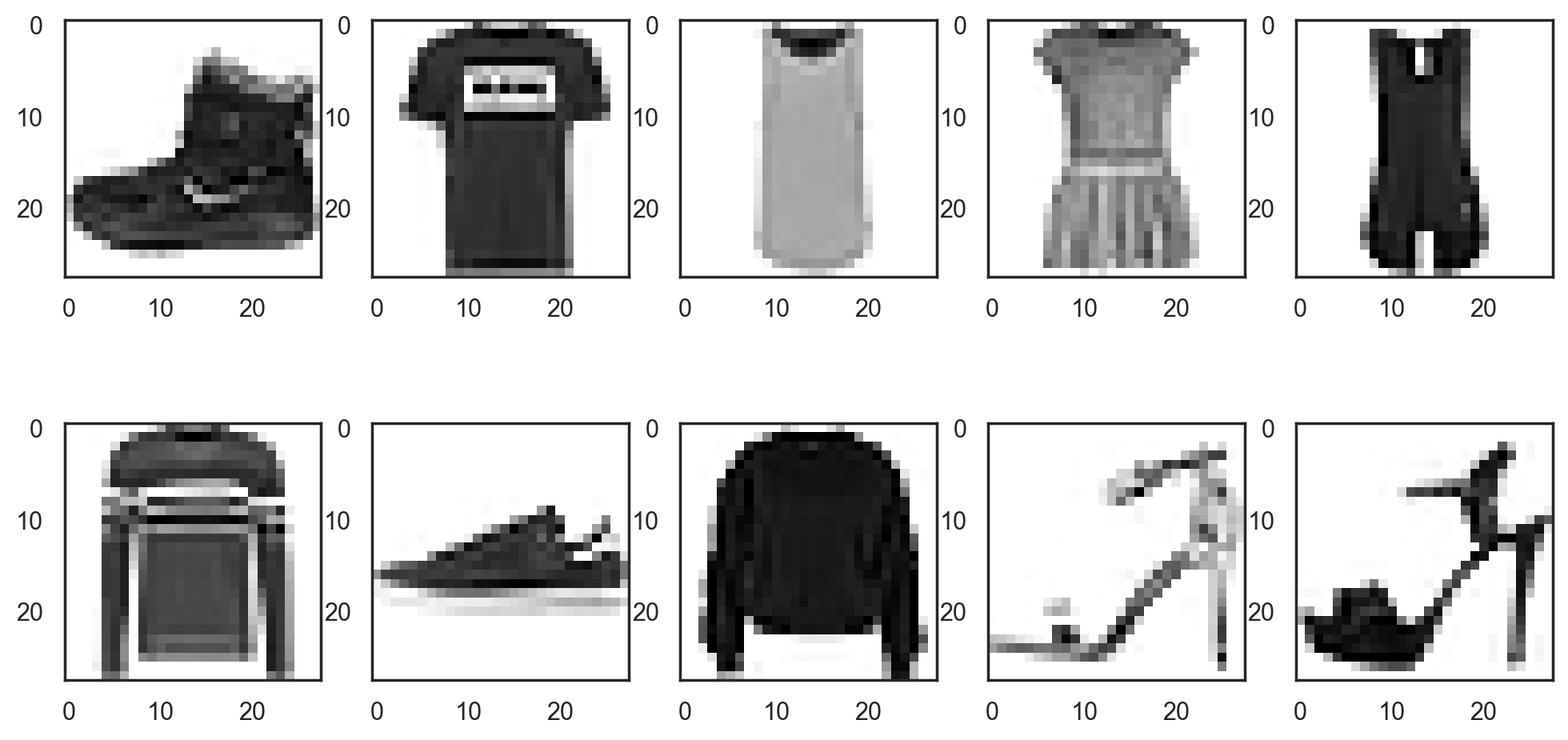
Example: training a CNN to recognize fashion items#
The Fashion-MNIST dataset contains 70,000 28x28 grayscale images of fashion items.
It is slightly more challenging than the ubiquitous MNIST handwritten digits dataset.
# Load the Fashion-MNIST digits dataset
(train_images, train_labels), (test_images, test_labels) = fashion_mnist.load_data()

print(f"Training images: {train_images.shape}. Training labels: {train_labels.shape}")
print(f"Test images: {test_images.shape}. Test labels: {test_labels.shape}")
Downloading data from https://storage.googleapis.com/tensorflow/tf-keras-datasets/train-labels-idx1-ubyte.gz
29515/29515 [==============================] - 0s 1us/step
Downloading data from https://storage.googleapis.com/tensorflow/tf-keras-datasets/train-images-idx3-ubyte.gz
26421880/26421880 [==============================] - 1s 0us/step
Downloading data from https://storage.googleapis.com/tensorflow/tf-keras-datasets/t10k-labels-idx1-ubyte.gz
5148/5148 [==============================] - 0s 0us/step
Downloading data from https://storage.googleapis.com/tensorflow/tf-keras-datasets/t10k-images-idx3-ubyte.gz
4422102/4422102 [==============================] - 0s 0us/step
Training images: (60000, 28, 28). Training labels: (60000,)
Test images: (10000, 28, 28). Test labels: (10000,)
# Plot the first 10 training images
with sns.axes_style("white"):  # Temporary hide Seaborn grid lines
    plt.figure(figsize=(12, 6))
    for i in range(10):
        image = train_images[i]
        fig = plt.subplot(2, 5, i + 1)
        plt.imshow(image, cmap=plt.cm.binary)
# Labels are integer scalars between 0 and 9
df_train_labels = pd.DataFrame(train_labels)
df_train_labels.columns = {"label"}
df_train_labels.sample(n=8)
| label | |
|---|---|
| 18079 | 0 |
| 17918 | 0 |
| 23857 | 2 |
| 10316 | 9 |
| 38185 | 1 |
| 867 | 9 |
| 40864 | 1 |
| 59097 | 8 |
Data preprocessing#
# Change pixel values from (0, 255) to (0, 1)
x_train = train_images.astype("float32") / 255
x_test = test_images.astype("float32") / 255

# Make sure images have shape (28, 28, 1) to apply convolution
x_train = np.expand_dims(x_train, -1)
x_test = np.expand_dims(x_test, -1)

# One-hot encoding of expected results
y_train = to_categorical(train_labels)
y_test = to_categorical(test_labels)

print(f"x_train: {x_train.shape}. y_train: {y_train.shape}")
print(f"x_test: {x_test.shape}. y_test: {y_test.shape}")
x_train: (60000, 28, 28, 1). y_train: (60000, 10)
x_test: (10000, 28, 28, 1). y_test: (10000, 10)
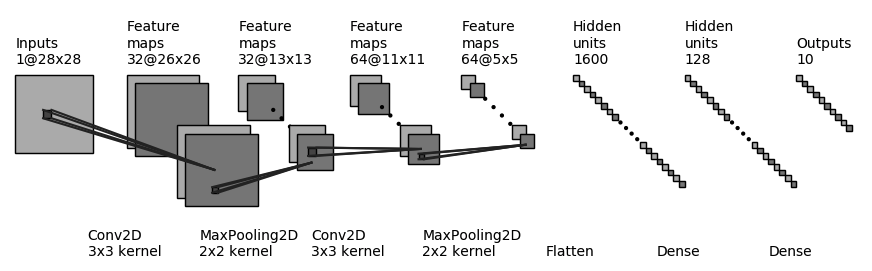
Expected convnet architecture#
# Create a linear stack of layers
cnn_model = Sequential()

# Convolution module 1: Conv2D+MaxPooling2D
#   filters: number of convolution filters
#   kernel_size: size of the convolution kernel (2D convolution window)
#   input_shape: shape of the input feature map
#   (Here, The expected input shape is a 3D tensor corresponding to an image)
cnn_model.add(
    Conv2D(filters=32, kernel_size=(3, 3), activation="relu", input_shape=(28, 28, 1))
)
#   pool_size: factors by which to downscale (vertical, horizontal)
cnn_model.add(MaxPooling2D(pool_size=(2, 2)))

# Convolution module 2
cnn_model.add(Conv2D(filters=64, kernel_size=(3, 3), activation="relu"))
cnn_model.add(MaxPooling2D(pool_size=(2, 2)))

# Flattening the last output feature map (a 3D tensor) to feed the Dense layer
cnn_model.add(Flatten())
cnn_model.add(Dense(128))
# To fight overfitting
cnn_model.add(Dropout(0.5))
# Classification layer
cnn_model.add(Dense(10, activation="softmax"))
Metal device set to: Apple M1 Pro
# Print model summary
cnn_model.summary()
Model: "sequential"
_________________________________________________________________
 Layer (type)                Output Shape              Param #
=================================================================
 conv2d (Conv2D)             (None, 26, 26, 32)        320

 max_pooling2d (MaxPooling2D  (None, 13, 13, 32)       0
 )

 conv2d_1 (Conv2D)           (None, 11, 11, 64)        18496

 max_pooling2d_1 (MaxPooling  (None, 5, 5, 64)         0
 2D)

 flatten (Flatten)           (None, 1600)              0

 dense (Dense)               (None, 128)               204928

 dropout (Dropout)           (None, 128)               0

 dense_1 (Dense)             (None, 10)                1290

=================================================================
Total params: 225,034
Trainable params: 225,034
Non-trainable params: 0
_________________________________________________________________
Convnet training#
# Preparing the model for training
cnn_model.compile(
    optimizer="adam", loss="categorical_crossentropy", metrics=["accuracy"]
)

# Training the model, using 10% of the training set for validation
# (May take several minutes depending on your system)
history = cnn_model.fit(
    x_train, y_train, epochs=10, verbose=2, batch_size=128, validation_split=0.1
)
Epoch 1/10
2023-05-25 19:39:05.028127: W tensorflow/tsl/platform/profile_utils/cpu_utils.cc:128] Failed to get CPU frequency: 0 Hz
422/422 - 10s - loss: 0.5622 - accuracy: 0.8018 - val_loss: 0.3639 - val_accuracy: 0.8688 - 10s/epoch - 23ms/step
Epoch 2/10
422/422 - 19s - loss: 0.3623 - accuracy: 0.8709 - val_loss: 0.3151 - val_accuracy: 0.8863 - 19s/epoch - 46ms/step
Epoch 3/10
422/422 - 6s - loss: 0.3202 - accuracy: 0.8854 - val_loss: 0.3032 - val_accuracy: 0.8895 - 6s/epoch - 14ms/step
Epoch 4/10
422/422 - 6s - loss: 0.2878 - accuracy: 0.8970 - val_loss: 0.2797 - val_accuracy: 0.8970 - 6s/epoch - 14ms/step
Epoch 5/10
422/422 - 6s - loss: 0.2686 - accuracy: 0.9036 - val_loss: 0.2714 - val_accuracy: 0.8997 - 6s/epoch - 14ms/step
Epoch 6/10
422/422 - 6s - loss: 0.2508 - accuracy: 0.9098 - val_loss: 0.2668 - val_accuracy: 0.9022 - 6s/epoch - 13ms/step
Epoch 7/10
422/422 - 6s - loss: 0.2346 - accuracy: 0.9155 - val_loss: 0.2638 - val_accuracy: 0.9062 - 6s/epoch - 14ms/step
Epoch 8/10
422/422 - 6s - loss: 0.2255 - accuracy: 0.9186 - val_loss: 0.2536 - val_accuracy: 0.9088 - 6s/epoch - 13ms/step
Epoch 9/10
422/422 - 6s - loss: 0.2130 - accuracy: 0.9228 - val_loss: 0.2568 - val_accuracy: 0.9048 - 6s/epoch - 14ms/step
Epoch 10/10
422/422 - 6s - loss: 0.2012 - accuracy: 0.9268 - val_loss: 0.2493 - val_accuracy: 0.9113 - 6s/epoch - 14ms/step
# Plot training history
plot_loss_acc(history)
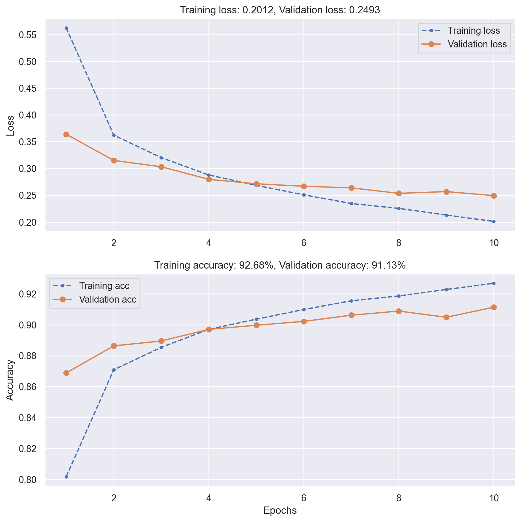
# Evaluate model performance on test data
_, test_acc = cnn_model.evaluate(x_test, y_test, verbose=0)

print(f"Test accuracy: {test_acc:.5f}")
Test accuracy: 0.90300
Using a pretrained convnet#
An efficient strategy#
A pretrained convnet is a saved network that was previously trained on a large dataset (typically on a large-scale image classification task). If the training set was general enough, it can act as a generic model and its learned features can be useful for many problems.
It is an example of transfer learning.
There are two ways to use a pretrained model: feature extraction and fine-tuning.
Feature extraction#
Reuse the convolution base of a pretrained model, and add a custom classifier trained from scratch on top ot if.
State-of-the-art models (VGG, ResNet, Inception…) are regularly published by top AI institutions.
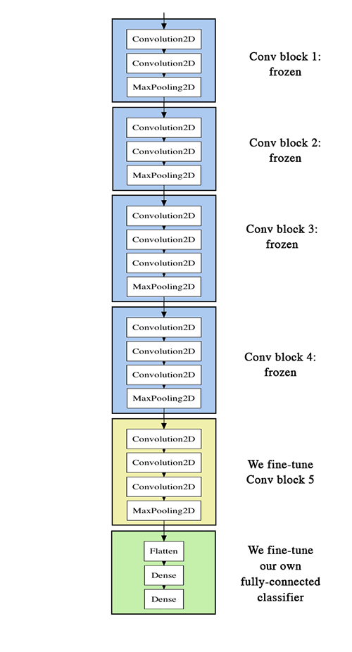
Fine-tuning#
Slightly adjusts the top feature extraction layers of the model being reused, in order to make it more relevant for the new context.
These top layers and the custom classification layers on top of them are jointly trained.
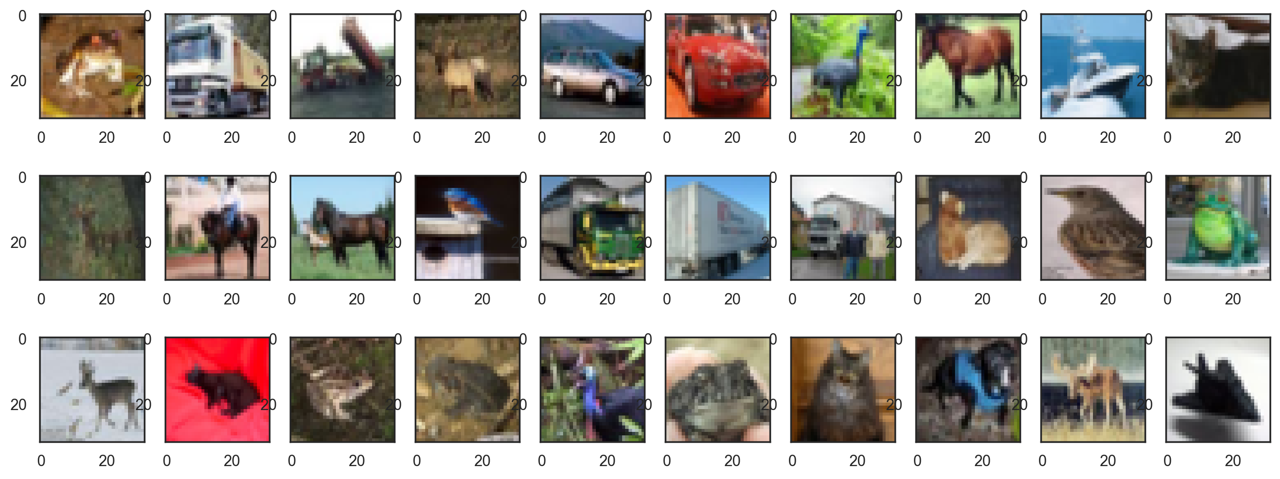
Example: using a pretrained convnet to recognize common objects#
The CIFAR10 dataset consists of 60,000 32x32 colour images in 10 classes, with 6,000 images per class. The classes are completely mutually exclusive.
There are 50,000 training images and 10,000 test images.
# Load the CIFAR10 dataset
(train_images, train_labels), (test_images, test_labels) = cifar10.load_data()

print(f"Training images: {train_images.shape}. Training labels: {train_labels.shape}")
print(f"Test images: {test_images.shape}. Test labels: {test_labels.shape}")
Downloading data from https://www.cs.toronto.edu/~kriz/cifar-10-python.tar.gz
170498071/170498071 [==============================] - 17s 0us/step
Training images: (50000, 32, 32, 3). Training labels: (50000, 1)
Test images: (10000, 32, 32, 3). Test labels: (10000, 1)
# Plot the first training images
with sns.axes_style("white"):  # Temporary hide Seaborn grid lines
    plt.figure(figsize=(16, 6))
    for i in range(30):
        image = train_images[i]
        fig = plt.subplot(3, 10, i + 1)
        plt.imshow(image, cmap=plt.cm.binary)
# Change pixel values from (0, 255) to (0, 1)
x_train = train_images.astype("float32") / 255
x_test = test_images.astype("float32") / 255

# One-hot encoding of expected results
y_train = to_categorical(train_labels)
y_test = to_categorical(test_labels)

print(f"x_train: {x_train.shape}. y_train: {y_train.shape}")
print(f"x_test: {x_test.shape}. y_test: {y_test.shape}")
x_train: (50000, 32, 32, 3). y_train: (50000, 10)
x_test: (10000, 32, 32, 3). y_test: (10000, 10)
# Using the convolutional base of VGG16
conv_base = VGG16(weights="imagenet", include_top=False, input_shape=(32, 32, 3))

# Freezing the convolutional base
# This prevents weight updates during training
conv_base.trainable = False

conv_base.summary()
Downloading data from https://storage.googleapis.com/tensorflow/keras-applications/vgg16/vgg16_weights_tf_dim_ordering_tf_kernels_notop.h5
58889256/58889256 [==============================] - 3s 0us/step
Model: "vgg16"
_________________________________________________________________
 Layer (type)                Output Shape              Param #
=================================================================
 input_1 (InputLayer)        [(None, 32, 32, 3)]       0

 block1_conv1 (Conv2D)       (None, 32, 32, 64)        1792

 block1_conv2 (Conv2D)       (None, 32, 32, 64)        36928

 block1_pool (MaxPooling2D)  (None, 16, 16, 64)        0

 block2_conv1 (Conv2D)       (None, 16, 16, 128)       73856

 block2_conv2 (Conv2D)       (None, 16, 16, 128)       147584

 block2_pool (MaxPooling2D)  (None, 8, 8, 128)         0

 block3_conv1 (Conv2D)       (None, 8, 8, 256)         295168

 block3_conv2 (Conv2D)       (None, 8, 8, 256)         590080

 block3_conv3 (Conv2D)       (None, 8, 8, 256)         590080

 block3_pool (MaxPooling2D)  (None, 4, 4, 256)         0

 block4_conv1 (Conv2D)       (None, 4, 4, 512)         1180160

 block4_conv2 (Conv2D)       (None, 4, 4, 512)         2359808

 block4_conv3 (Conv2D)       (None, 4, 4, 512)         2359808

 block4_pool (MaxPooling2D)  (None, 2, 2, 512)         0

 block5_conv1 (Conv2D)       (None, 2, 2, 512)         2359808

 block5_conv2 (Conv2D)       (None, 2, 2, 512)         2359808

 block5_conv3 (Conv2D)       (None, 2, 2, 512)         2359808

 block5_pool (MaxPooling2D)  (None, 1, 1, 512)         0

=================================================================
Total params: 14,714,688
Trainable params: 0
Non-trainable params: 14,714,688
_________________________________________________________________
# Create our new model
pretrained_cnn_model = Sequential()
# Add VGG as its base
pretrained_cnn_model.add(conv_base)
# Add a Dense classifier on top of the pretrained base
pretrained_cnn_model.add(Flatten())
pretrained_cnn_model.add(Dense(512, activation="relu"))
pretrained_cnn_model.add(Dropout(0.5))
pretrained_cnn_model.add(Dense(10, activation="softmax"))

pretrained_cnn_model.summary()
Model: "sequential_1"
_________________________________________________________________
 Layer (type)                Output Shape              Param #
=================================================================
 vgg16 (Functional)          (None, 1, 1, 512)         14714688

 flatten_1 (Flatten)         (None, 512)               0

 dense_2 (Dense)             (None, 512)               262656

 dropout_1 (Dropout)         (None, 512)               0

 dense_3 (Dense)             (None, 10)                5130

=================================================================
Total params: 14,982,474
Trainable params: 267,786
Non-trainable params: 14,714,688
_________________________________________________________________
# Preparing the model for training
pretrained_cnn_model.compile(
    optimizer="adam", loss="categorical_crossentropy", metrics=["accuracy"]
)

# Training the model, using 10% of the training set for validation
# (May take several minutes depending on your system)
history = pretrained_cnn_model.fit(
    x_train, y_train, epochs=20, verbose=1, batch_size=32, validation_split=0.1
)
Epoch 1/20
1407/1407 [==============================] - 19s 13ms/step - loss: 1.4967 - accuracy: 0.4814 - val_loss: 1.2548 - val_accuracy: 0.5634
Epoch 2/20
1407/1407 [==============================] - 19s 13ms/step - loss: 1.3561 - accuracy: 0.5318 - val_loss: 1.2202 - val_accuracy: 0.5736
Epoch 3/20
1407/1407 [==============================] - 18s 13ms/step - loss: 1.3405 - accuracy: 0.5387 - val_loss: 1.2391 - val_accuracy: 0.5684
Epoch 4/20
1407/1407 [==============================] - 17s 12ms/step - loss: 1.3481 - accuracy: 0.5392 - val_loss: 1.2275 - val_accuracy: 0.5690
Epoch 5/20
1407/1407 [==============================] - 17s 12ms/step - loss: 1.3426 - accuracy: 0.5392 - val_loss: 1.2746 - val_accuracy: 0.5538
Epoch 6/20
1407/1407 [==============================] - 17s 12ms/step - loss: 1.3436 - accuracy: 0.5402 - val_loss: 1.2272 - val_accuracy: 0.5734
Epoch 7/20
1407/1407 [==============================] - 18s 13ms/step - loss: 1.3579 - accuracy: 0.5374 - val_loss: 1.2734 - val_accuracy: 0.5550
Epoch 8/20
1407/1407 [==============================] - 18s 13ms/step - loss: 1.3506 - accuracy: 0.5417 - val_loss: 1.2168 - val_accuracy: 0.5750
Epoch 9/20
1407/1407 [==============================] - 17s 12ms/step - loss: 1.3558 - accuracy: 0.5417 - val_loss: 1.2757 - val_accuracy: 0.5486
Epoch 10/20
1407/1407 [==============================] - 18s 13ms/step - loss: 1.3611 - accuracy: 0.5412 - val_loss: 1.2390 - val_accuracy: 0.5664
Epoch 11/20
1407/1407 [==============================] - 17s 12ms/step - loss: 1.3693 - accuracy: 0.5412 - val_loss: 1.2821 - val_accuracy: 0.5622
Epoch 12/20
1407/1407 [==============================] - 18s 13ms/step - loss: 1.3772 - accuracy: 0.5366 - val_loss: 1.2726 - val_accuracy: 0.5660
Epoch 13/20
1407/1407 [==============================] - 18s 13ms/step - loss: 1.3785 - accuracy: 0.5385 - val_loss: 1.3005 - val_accuracy: 0.5568
Epoch 14/20
1407/1407 [==============================] - 18s 13ms/step - loss: 1.3975 - accuracy: 0.5342 - val_loss: 1.2803 - val_accuracy: 0.5722
Epoch 15/20
1407/1407 [==============================] - 18s 13ms/step - loss: 1.3994 - accuracy: 0.5356 - val_loss: 1.2798 - val_accuracy: 0.5658
Epoch 16/20
1407/1407 [==============================] - 17s 12ms/step - loss: 1.4084 - accuracy: 0.5348 - val_loss: 1.2851 - val_accuracy: 0.5544
Epoch 17/20
1407/1407 [==============================] - 17s 12ms/step - loss: 1.4200 - accuracy: 0.5312 - val_loss: 1.2668 - val_accuracy: 0.5604
Epoch 18/20
1407/1407 [==============================] - 17s 12ms/step - loss: 1.4212 - accuracy: 0.5348 - val_loss: 1.3595 - val_accuracy: 0.5426
Epoch 19/20
1407/1407 [==============================] - 18s 13ms/step - loss: 1.4391 - accuracy: 0.5298 - val_loss: 1.2996 - val_accuracy: 0.5550
Epoch 20/20
1407/1407 [==============================] - 18s 13ms/step - loss: 1.4372 - accuracy: 0.5292 - val_loss: 1.3527 - val_accuracy: 0.5308
# Plot training history
plot_loss_acc(history)
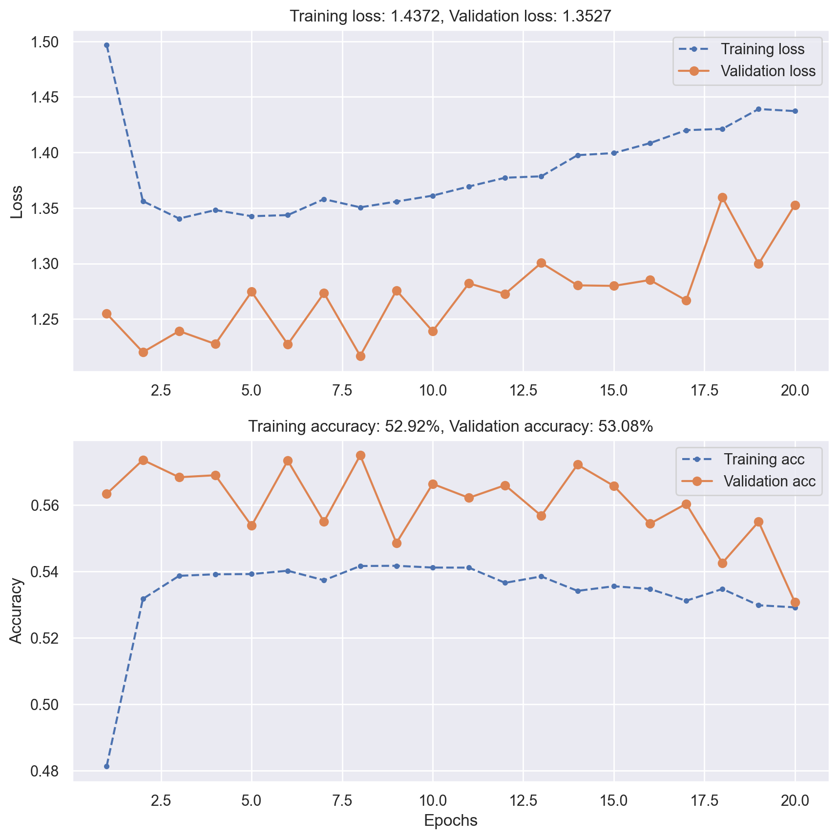
# Evaluate model performance on test data
_, test_acc = pretrained_cnn_model.evaluate(x_test, y_test, verbose=0)

print(f"Test accuracy: {test_acc:.5f}")
Test accuracy: 0.51820