Logistic Regression

Logistic Regression#

Environment setup#

import platform

print(f"Python version: {platform.python_version()}")
assert platform.python_version_tuple() >= ("3", "6")

import numpy as np
import matplotlib
import matplotlib.pyplot as plt
from matplotlib.colors import ListedColormap
import seaborn as sns

Python version: 3.7.5

# Setup plots
%matplotlib inline
plt.rcParams["figure.figsize"] = 10, 8
%config InlineBackend.figure_format = 'retina'
sns.set()

import sklearn

print(f"scikit-learn version: {sklearn.__version__}")
assert sklearn.__version__ >= "0.20"

from sklearn.datasets import make_classification, make_blobs
from sklearn.linear_model import SGDClassifier, LogisticRegression
from sklearn.metrics import classification_report

scikit-learn version: 0.22.1

Binary classification#

Problem formulation#

Logistic regression is a classification algorithm used to estimate the probability that a data sample belongs to a particular class.

A logistic regression model computes a weighted sum of the input features (plus a bias term), then applies the logistic function to this sum in order to output a probability.

y^{'} = h_{θ} (x x) = σ (θ θ^{T} x x)

The function output is thresholded to form the model’s prediction:

$0$ if $y^{'} < 0.5$
$1$ if $y^{'} ⩾ 0.5$

Loss function: Binary Crossentropy (log loss)#

See loss definition for details.

Model training#

No analytical solution because of the non-linear $σ ()$ function: gradient descent is the only option.
Since the loss function is convex, GD (with the right hyperparameters) is guaranteed to find the global loss minimum.
Different GD optimizers exist: newton-cg, l-bfgs, sag… Stochastic gradient descent is another possibility, efficient for large numbers of samples and features.

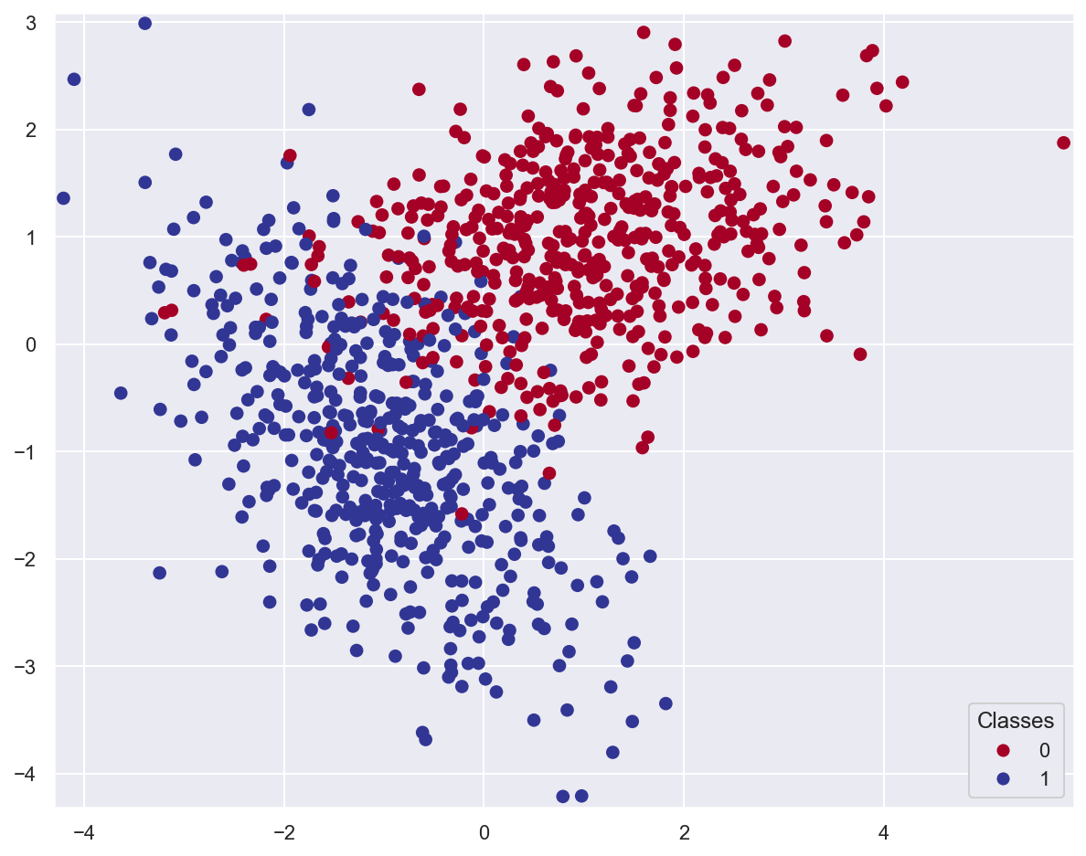
\begin{array}{r} \nabla_{θ} L (θ θ) = (\begin{array}{c} \frac{\partial}{\partial θ_{0}} L (θ) \\ \frac{\partial}{\partial θ_{1}} L (θ) \\ ⋮ \\ \frac{\partial}{\partial θ_{n}} L (θ) \end{array}) = \frac{2}{m} X X^{T} (σ (X X θ θ) - y y) \end{array}

Example: classify planar data#

# Generate 2 classes of linearly separable data
x_train, y_train = make_classification(
    n_samples=1000,
    n_features=2,
    n_redundant=0,
    n_informative=2,
    random_state=26,
    n_clusters_per_class=1,
)
plot_data(x_train, y_train)

../_images/e27ec2d6477d6d6cf8eeb2c51c8a609fa713fab37e29f1c2be1c93fe792aec2a.png

# Create a Logistic Regression model based on stochastic gradient descent
# Alternative: using the LogisticRegression class which implements many GD optimizers
lr_model = SGDClassifier(loss="log")

# Train the model
lr_model.fit(x_train, y_train)

print(f"Model weights: {lr_model.coef_}, bias: {lr_model.intercept_}")

Model weights: [[-2.96719034 -2.55668143]], bias: [-0.57585284]

# Print report with classification metrics
print(classification_report(y_train, lr_model.predict(x_train)))

              precision    recall  f1-score   support

           0       0.96      0.92      0.94       502
           1       0.92      0.96      0.94       498

    accuracy                           0.94      1000
   macro avg       0.94      0.94      0.94      1000
weighted avg       0.94      0.94      0.94      1000

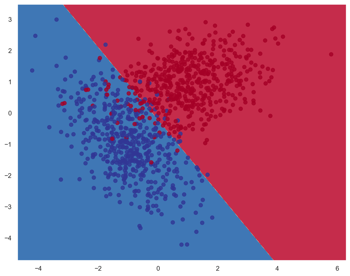
# Plot decision boundary
plot_decision_boundary(lambda x: lr_model.predict(x), x_train, y_train)

../_images/d1e1f5b2e8328fa6a0d60efd07cf24642fbc78b93d53951e890e53b7775f4266.png

Multivariate regression#

Problem formulation#

Multivariate regression, also called softmax regression, is a generalization of logistic regression for multiclass classification.

A softmax regression model computes the scores $s_{k} (x x)$ for each class $k$ , then estimates probabilities for each class by applying the softmax function to compute a probability distribution.

For a sample $x x^{(i)}$ , the model predicts the class $k$ that has the highest probability.

s_{k} (x x) = {θ θ^{(k)}}^{T} x x

prediction = \underset{k}{argmax} σ (s (x x^{(i)}))_{k}

Each class $k$ has its own parameter vector $θ θ^{(k)}$ .

Model output#

$y y^{(i)}$ (ground truth): binary vector of $K$ values. $y_{k}^{(i)}$ is equal to 1 if the $i$ th sample’s class corresponds to $k$ , 0 otherwise.
$y y^{' (i)}$ : probability vector of $K$ values, computed by the model. $y_{k}^{' (i)}$ represents the probability that the $i$ th sample belongs to class $k$ .

\begin{array}{r} y y^{(i)} = (\begin{array}{c} y_{1}^{(i)} \\ y_{2}^{(i)} \\ ⋮ \\ y_{K}^{(i)} \end{array}) \in R R^{K} y y^{' (i)} = (\begin{array}{c} y_{1}^{' (i)} \\ y_{2}^{' (i)} \\ ⋮ \\ y_{K}^{' (i)} \end{array}) = (\begin{array}{c} σ (s (x x^{(i)}))_{1} \\ σ (s (x x^{(i)}))_{2} \\ ⋮ \\ σ (s (x x^{(i)}))_{K} \end{array}) \in R R^{K} \end{array}

Loss function: Categorical Crossentropy#

See loss definition for details.

Model training#

Via gradient descent:

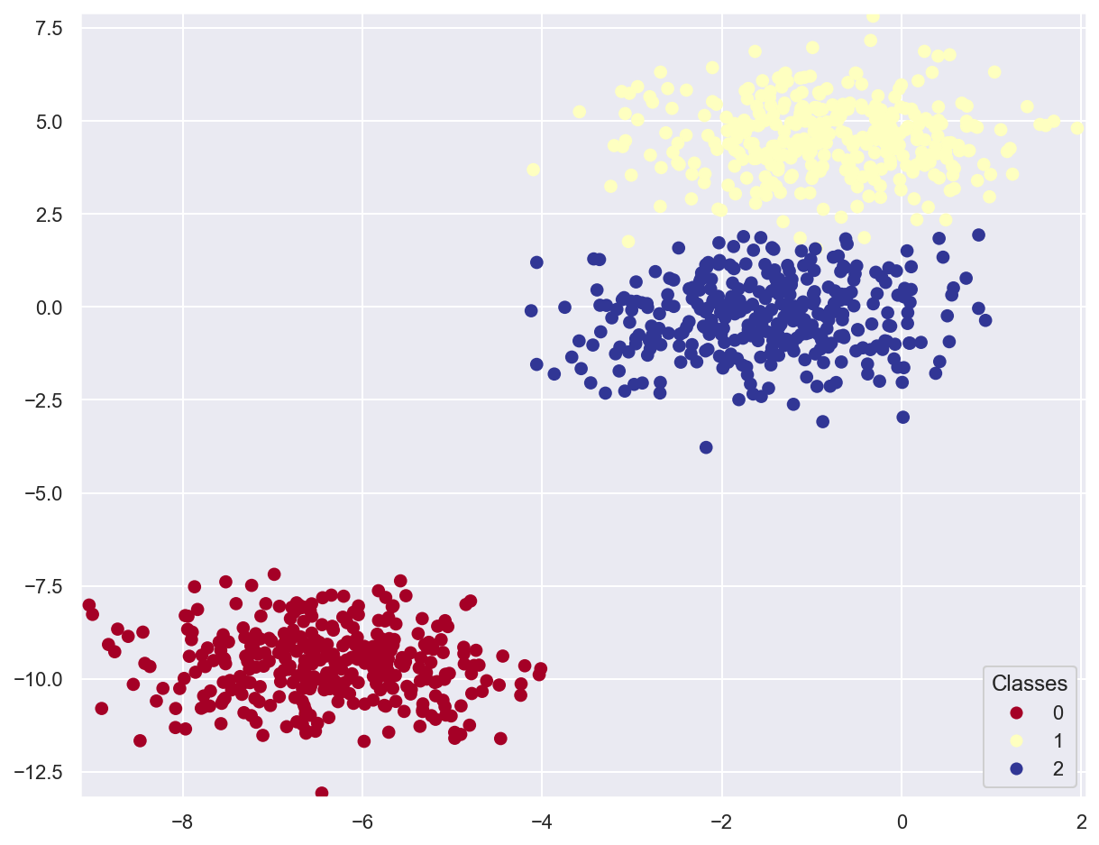
\nabla_{θ^{(k)}} L (θ θ) = \frac{1}{m} \sum_{i = 1}^{m} (y_{k}^{' (i)} - y_{k}^{(i)}) x x^{(i)}

θ θ_{n e x t}^{(k)} = θ θ^{(k)} - η \nabla_{θ^{(k)}} L (θ θ)

Example: classify multiclass planar data#

# Generate 3 classes of linearly separable data
x_train_multi, y_train_multi = make_blobs(n_samples=1000, n_features=2, centers=3, random_state=11)

plot_data(x_train_multi, y_train_multi)

../_images/2861ea21654fad907d37af8fd2ceef6539be231b96a8c488d5219f49a7650729.png

# Create a Logistic Regression model based on stochastic gradient descent
# Alternative: using LogisticRegression(multi_class="multinomial") which implements SR
lr_model_multi = SGDClassifier(loss="log")

# Train the model
lr_model_multi.fit(x_train_multi, y_train_multi)

print(f"Model weights: {lr_model_multi.coef_}, bias: {lr_model_multi.intercept_}")

Model weights: [[ -5.76624648 -17.43149458]
 [ -1.27339599  19.17812979]
 [  1.5231193   -0.91647832]], bias: [-133.15588019  -38.36388245    2.53712564]

# Print report with classification metrics
print(classification_report(y_train_multi, lr_model_multi.predict(x_train_multi)))

              precision    recall  f1-score   support

           0       1.00      1.00      1.00       334
           1       0.99      0.99      0.99       333
           2       0.99      0.99      0.99       333

    accuracy                           0.99      1000
   macro avg       0.99      0.99      0.99      1000
weighted avg       1.00      0.99      0.99      1000

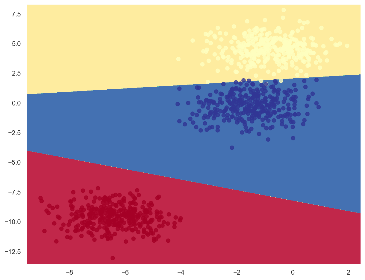
# Plot decision boundaries
plot_decision_boundary(lambda x: lr_model_multi.predict(x), x_train_multi, y_train_multi)

../_images/2810f376bb0f6f4245283fffe244c5853bb49c46cf02b771d7ba9161cfa30f40.png

Logistic Regression

Contents

Logistic Regression#

Environment setup#

Binary classification#

Problem formulation#

Loss function: Binary Crossentropy (log loss)#

Model training#

Example: classify planar data#

Multivariate regression#

Problem formulation#

Model output#

Loss function: Categorical Crossentropy#

Model training#

Example: classify multiclass planar data#