Recurrent Neural Networks

Summary

• RNN fundamentals

• LSTM, GRU and 1D convolutions

RNN fundamentals

(Heavily inspired by Chapter 15 of Hands-On Machine Learning by Aurélien Géron)

Recurrent Neural Networks in a nutshell

• Family of neural networks that maintain some kind of state, contrary to feedforward networks like MLP.

• Able to handle sequential data (data for which there is some sort of dependency through time).

• Can process input of arbitrary length.

• Useful in many contexts:

  • Time series analysis.

  • Natural Language Processing.

  • Audio tasks (text-to-speech, speech-to-text, music generation).

  • …

Terminology

• Sequence: instance of sequential data.

• Time step (or frame): incremental change in time used to discretize the sequence.

• Cell: recurrent unit in a RNN.

• Unrolling: representing the RNN flow against the time axis.

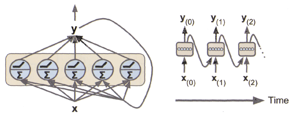
RNN architecture

RNN have loops into them, allowing information to persist and be passed from one step of the network to the next.

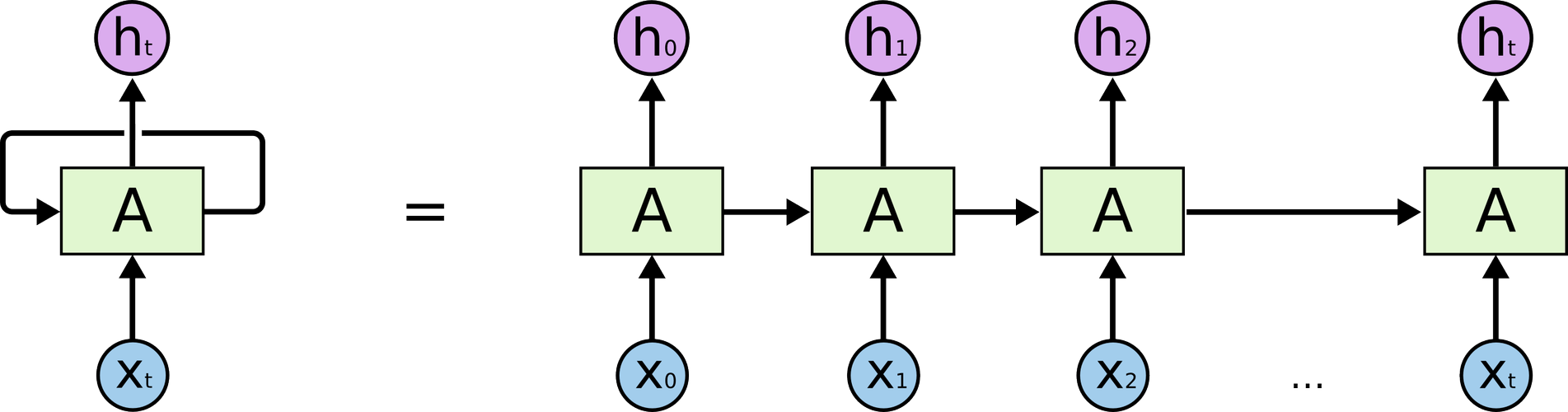
At each time step, the output is a function of all inputs from previous time steps. The network has a form of memory, encoding information about the timesteps it has seen so far.

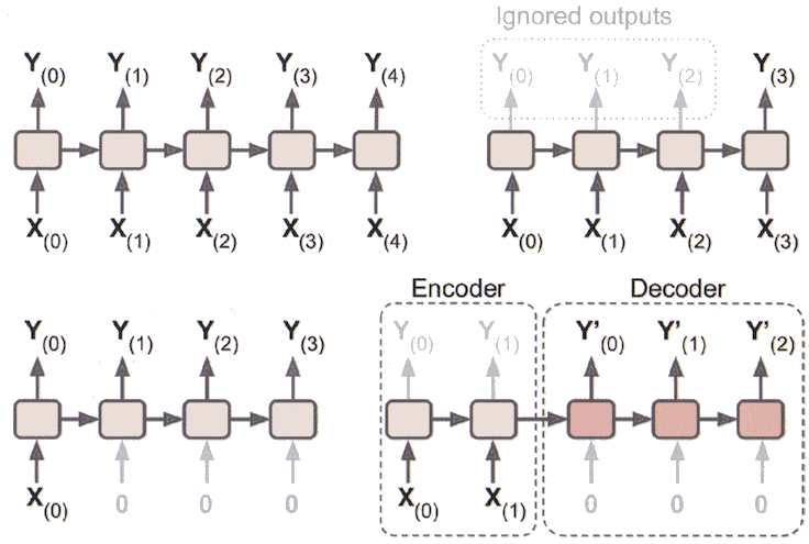
Typology of RNNs

RNN Type	In	Out
Sequence-to-sequence	An input sequence	An output sequence
Sequence-to-vector	An input sequence	Value of output sequence for last timestep
Vector-to-sequence	Single value of input sequence	An output sequence
Encoder-decoder	An input sequence	An output sequence, after encoding (seq2vec) and decoding (vec2seq)

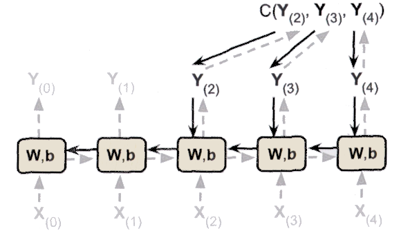
Training a RNN

A RNN is similar to a feedforward neural network that has a layer for each time step. Its weights are shared across time.

The training process uses backpropagation through time (BPTT). After the forward pass, gradients of the cost function are propagated backwards through the unrolled network (more details).

Sequence format

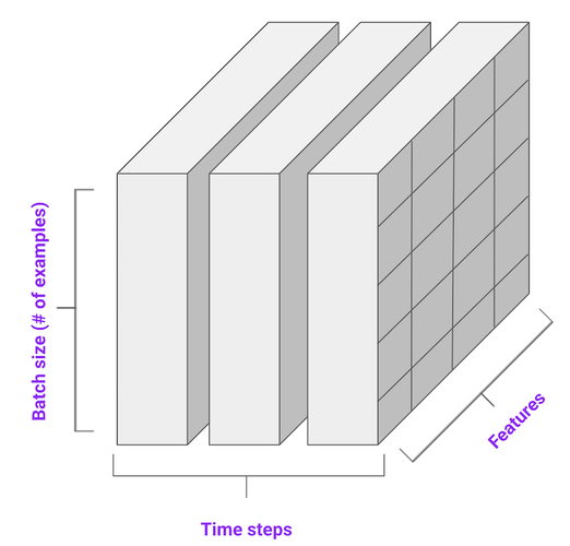
Input sequences for a RNN are 3D tensors. Axis are: batch size (number of sequences in the batch), time steps for each sequence, and features (values of attributes at a specific time step).

• An univariate sequence has only a single feature per time step.

• A multivariate sequence has several features per time step.

Example: forecasting a univariate time series

Environment setup

import platform

print(f"Python version: {platform.python_version()}")
assert platform.python_version_tuple() >= ("3", "6")

import numpy as np
import matplotlib.pyplot as plt
import seaborn as sns

Python version: 3.7.5

# Setup plots
%matplotlib inline
plt.rcParams["figure.figsize"] = 10, 8
%config InlineBackend.figure_format = "retina"
sns.set()

import tensorflow as tf

print(f"TensorFlow version: {tf.__version__}")
print(f"Keras version: {tf.keras.__version__}")

from tensorflow.keras.losses import mean_squared_error
from tensorflow.keras.models import Sequential
from tensorflow.keras.layers import SimpleRNN, Dense, LSTM, GRU, Conv1D
from tensorflow.keras.optimizers import Adam

TensorFlow version: 2.0.0
Keras version: 2.2.4-tf

Show code cell source Hide code cell source

# Utility functions
# First two are adapted from
# https://github.com/ageron/handson-ml2/blob/master/15_processing_sequences_using_rnns_and_cnns.ipynb


def generate_time_series(batch_size, n_steps):
    """Generate a batch of time series with same length = n_steps
    Each series is the sum of two sine waves of fixed amplitudes 
        but random frequencies and phases, with added noise
    Return a 3D tensor of shape (batch_size, n_steps, 1)"""

    freq1, freq2, offsets1, offsets2 = np.random.rand(4, batch_size, 1)
    time = np.linspace(0, 1, n_steps)
    series = 0.5 * np.sin((time - offsets1) * (freq1 * 10 + 10))  #   wave 1
    series += 0.2 * np.sin((time - offsets2) * (freq2 * 20 + 20))  # + wave 2
    series += 0.1 * (np.random.rand(batch_size, n_steps) - 0.5)  # + noise
    return series[..., np.newaxis].astype(np.float32)


def plot_series(series, y_true, y_pred=None, x_label="$t$", y_label="$x(t)$"):
    """Plot a time series with actual and predicted future values
    series: vector of shape (time steps, )
    y_true: scalar (if only 1 ahead step) or vector of shape (ahead steps,)
    y_pred: scalar (if only 1 ahead step) or vector of shape (ahead steps,)"""

    plt.plot(series, ".-")
    n_steps = series.shape[0]

    # Calculate the number of steps ahead (= number of future values)
    n_steps_ahead = 1
    if not np.isscalar(y_true):
        n_steps_ahead = y_true.shape[0]

    # Plot actual future values
    plt.plot(np.arange(n_steps, n_steps + n_steps_ahead), y_true, "ro-", label="Actual")

    if y_pred is not None:
        # Plot predicted future values
        plt.plot(
            np.arange(n_steps, n_steps + n_steps_ahead),
            y_pred,
            "bx-",
            label="Predicted",
            markersize=10,
        )
    if x_label:
        plt.xlabel(x_label, fontsize=16)
    if y_label:
        plt.ylabel(y_label, fontsize=16, rotation=0)

    plt.hlines(0, 0, 100, linewidth=1)
    plt.axis([0, n_steps + n_steps_ahead, -1, 1])
    plt.legend(fontsize=14)


def plot_loss(history):
    """Plot training loss for a Keras model
    Takes a Keras History object as parameter"""

    loss = history.history["loss"]
    epochs = range(1, len(loss) + 1)

    plt.figure(figsize=(10, 5))
    plt.plot(epochs, loss, ".--", label="Training loss")
    final_loss = loss[-1]
    title = "Training loss: {:.4f}".format(final_loss)
    plt.ylabel("Loss")
    if "val_loss" in history.history:
        val_loss = history.history["val_loss"]
        plt.plot(epochs, val_loss, "o-", label="Validation loss")
        final_val_loss = val_loss[-1]
        title += ", Validation loss: {:.4f}".format(final_val_loss)
    plt.title(title)
    plt.legend()

# Generate a batch of time series
n_steps = 50
series = generate_time_series(10000, n_steps + 1)

print(f"series: {series.shape}")

# Split dataset as usual between train/validation/test sets
# -1 is used to retrieve feature(s) for last time step only (the one we try to predict)
x_train, y_train = series[:7000, :n_steps], series[:7000, -1]
x_val, y_val = series[7000:9000, :n_steps], series[7000:9000, -1]
x_test, y_test = series[9000:, :n_steps], series[9000:, -1]

print(f"x_train: {x_train.shape}, y_train: {y_train.shape}")
print(f"x_val: {x_val.shape}, y_val: {y_val.shape}")
print(f"x_test: {x_test.shape}, y_test: {y_test.shape}")

series: (10000, 51, 1)
x_train: (7000, 50, 1), y_train: (7000, 1)
x_val: (2000, 50, 1), y_val: (2000, 1)
x_test: (1000, 50, 1), y_test: (1000, 1)

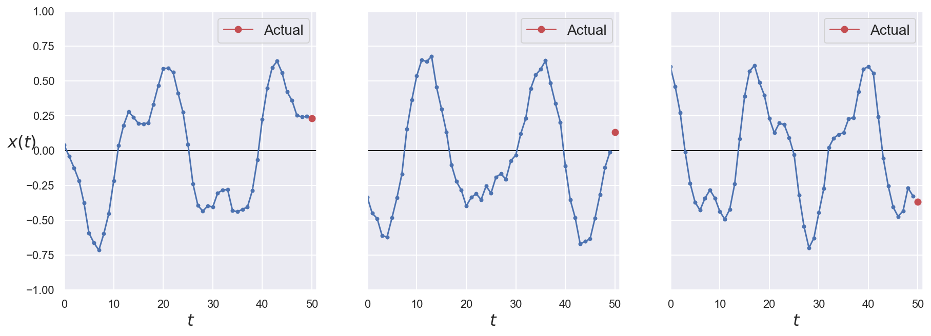
# Plot 3 series from the validation set
fig, axes = plt.subplots(nrows=1, ncols=3, sharey=True, figsize=(15, 5))
for col in range(3):
    plt.sca(axes[col])
    plot_series(
        series=x_val[col, :, 0],
        y_true=y_val[col, 0],
        y_label=("$x(t)$" if col == 0 else None),
    )
plt.show()

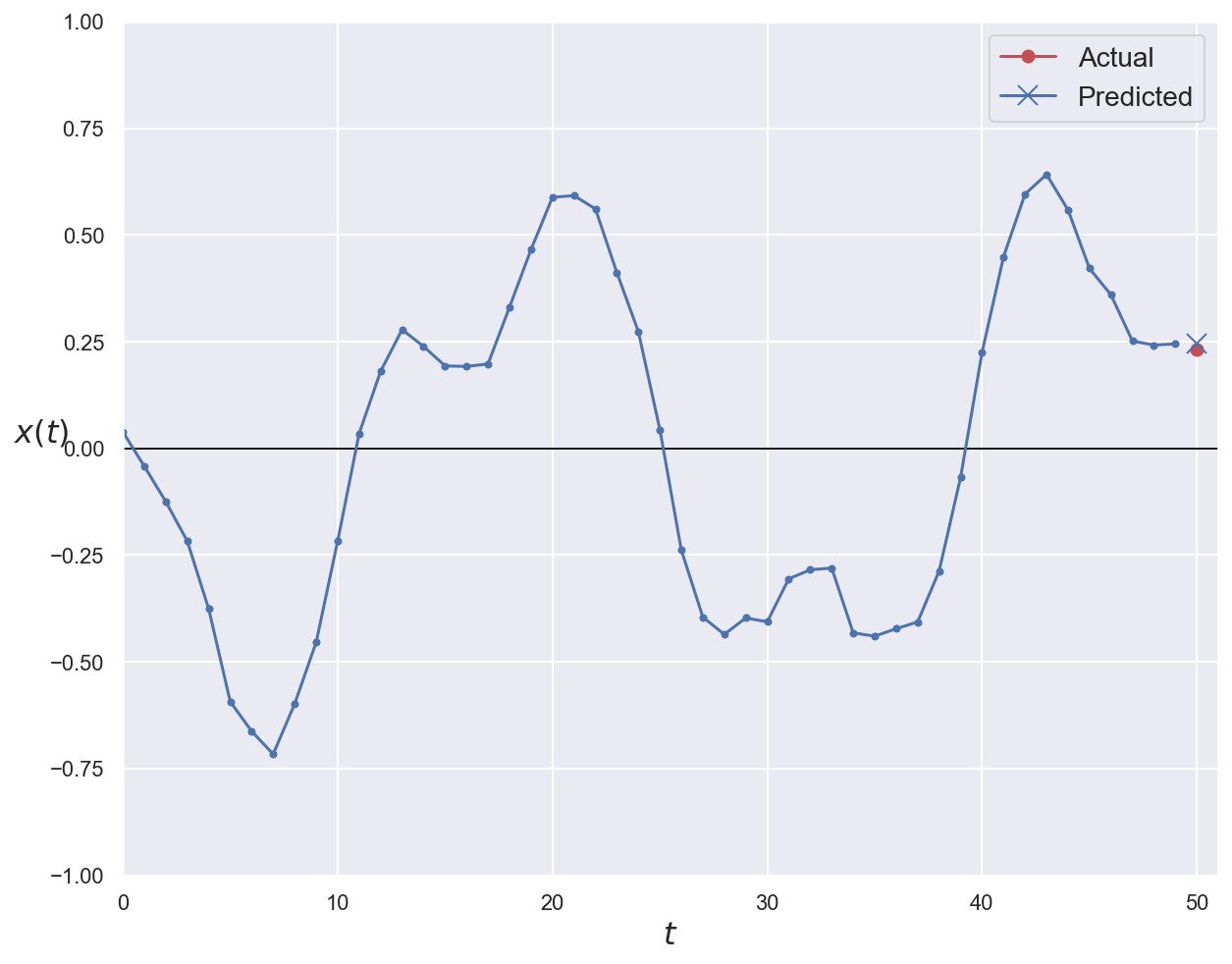
Single step, naïve forecasting

Here, we only try to predict the sequence value one step ahead in the future.

A baseline solution (always useful at the beginning of any ML project) would be to use the last know value as prediction.

# Naïve prediction = input for last time step
y_pred_naive = x_val[:, -1]
print(f"y_pred_naive: {y_pred_naive.shape}")

print(f"Naïve predictor MSE: {np.mean(mean_squared_error(y_val, y_pred_naive)):0.05f}")

y_pred_naive: (2000, 1)
Naïve predictor MSE: 0.02044

# Plot first validation series with ground truth and prediction
plot_series(series=x_val[0, :, 0], y_true=y_val[0, 0], y_pred=y_pred_naive[0, 0])
plt.show()

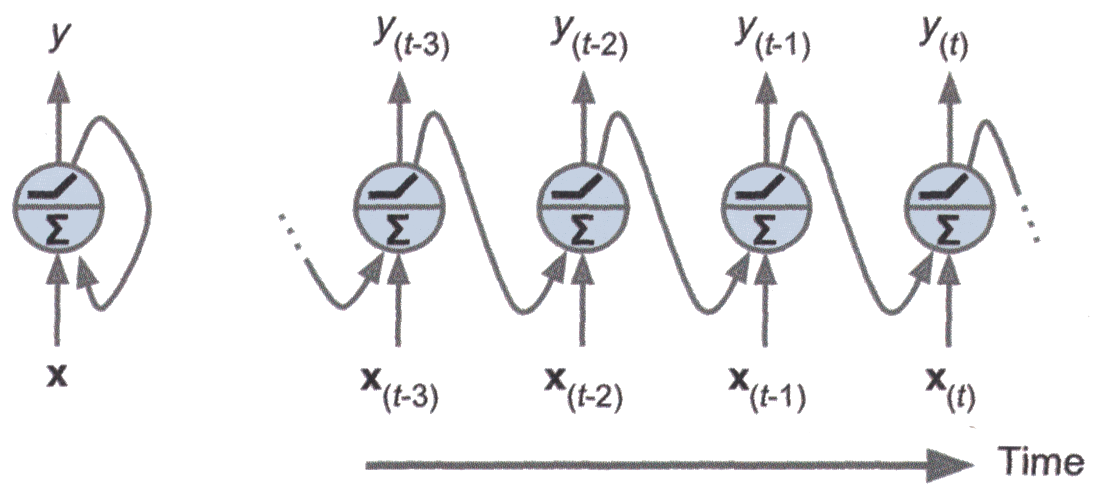
Recurrent neurons

The most basic form of RNN cell is a recurrent neuron. It simply sends its output back to itself.

At each time step \(t\), it receives the input vector \(\mathbf{x}_{(t)}\) and its own scalar output from the previous time step, \(y_{(t-1)}\).

# Create a linear stack of layers
basic_rnn_model = Sequential()

# Add a RNN layer to the model
# units: dimensionality of the output space (= number of cells inside the layer)
# input_shape: dimensionality of input, excluding batch dimension: vector of shape (time steps, features)
#   Could also be (n_steps, 1) here, but RNN can process any number of time steps, so None is also ok
# This layer expects input as a 3D tensor (batch size, time steps, features)
# Output shape is a 2D tensor (batch size, units) corresponding to the last time step
# Activation function is tanh by default
basic_rnn_model.add(SimpleRNN(units=1, input_shape=(None, 1)))

# 1 weight for input, 1 for recurrent output, 1 for bias = 3 parameters
basic_rnn_model.summary()

Model: "sequential"
_________________________________________________________________
Layer (type)                 Output Shape              Param #   
=================================================================
simple_rnn (SimpleRNN)       (None, 1)                 3         
=================================================================
Total params: 3
Trainable params: 3
Non-trainable params: 0
_________________________________________________________________

# Compile and train the model

basic_rnn_model.compile(optimizer=Adam(lr=0.005), loss="mse")

history = basic_rnn_model.fit(
    x_train, y_train, epochs=15, verbose=0, validation_data=(x_val, y_val)
)

plot_loss(history)

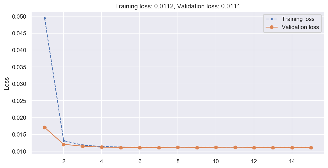
# Compute predictions and error on validation data

y_pred_basic = basic_rnn_model.predict(x_val)

print(f"Basic RNN MSE: {np.mean(mean_squared_error(y_val, y_pred_basic)):0.05f}")

Basic RNN MSE: 0.01113

# Plot first validation series with ground truth and prediction
plot_series(series=x_val[0, :, 0], y_true=y_val[0, 0], y_pred=y_pred_basic[0, 0])
plt.show()

Recurrent layers

Recurrent neurons can be stacked together to form a recurrent layer.

At each time step \(t\), each neuron of the layer receives both the input vector \(\mathbf{x}_{(t)}\) and the output of the layer from the previous time step, \(\mathbf{y}_{(t-1)}\) (which is a vector in that case).

stacked_rnn_model = Sequential()

# return_sequences: if True, the layer outputs the whole sequence instead of the value for last time step
# In that case, output shape is a 3D tensor (batch size, time steps, units)
# This is needed to connect this layer to other recurrent layers
stacked_rnn_model.add(SimpleRNN(units=20, return_sequences=True, input_shape=(None, 1)))

# return_sequences is False by default
# In that case, output shape is a 2D tensor (batch size, units)
# Here, we only care about output for the last time step
stacked_rnn_model.add(SimpleRNN(units=20))

# Add a linear layer to compute the prediction
stacked_rnn_model.add(Dense(units=1))

# First RNN layer: 20 (input) + 20 (bias) + 20x20 (recurrent output) = 440 parameters
# Second RNN layer: 20x20 (input) + 20x20 (recurrent output) + 20 (bias) = 820 parameters
# Dense layer: 20 (input) + 1 (bias) = 21 parameters
stacked_rnn_model.summary()

Model: "sequential_1"
_________________________________________________________________
Layer (type)                 Output Shape              Param #   
=================================================================
simple_rnn_1 (SimpleRNN)     (None, None, 20)          440       
_________________________________________________________________
simple_rnn_2 (SimpleRNN)     (None, 20)                820       
_________________________________________________________________
dense (Dense)                (None, 1)                 21        
=================================================================
Total params: 1,281
Trainable params: 1,281
Non-trainable params: 0
_________________________________________________________________

# Compile and train the model

stacked_rnn_model.compile(optimizer="adam", loss="mse")

history = stacked_rnn_model.fit(
    x_train, y_train, epochs=15, verbose=0, validation_data=(x_val, y_val)
)

plot_loss(history)

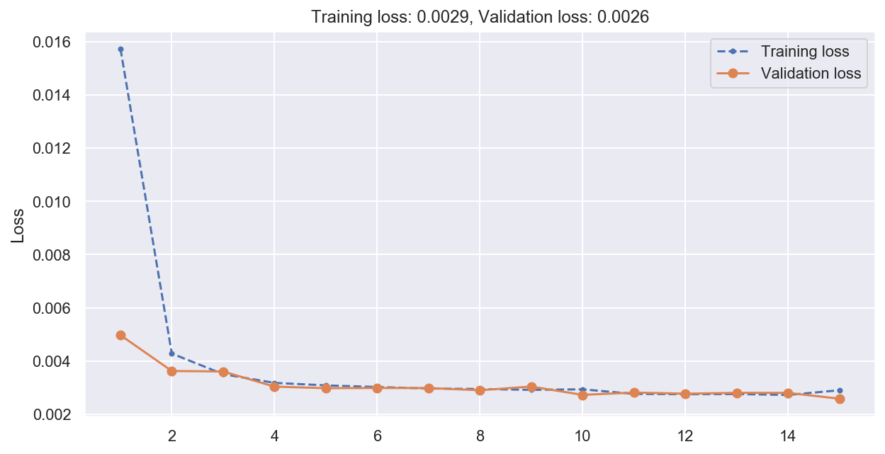
# Compute predictions and error on validation data

y_pred_stacked = stacked_rnn_model.predict(x_val)

print(f"Stacked RNN MSE: {np.mean(mean_squared_error(y_val, y_pred_stacked)):0.05f}")

Stacked RNN MSE: 0.00259

# Plot first validation series with ground truth and prediction
plot_series(series=x_val[0, :, 0], y_true=y_val[0, 0], y_pred=y_pred_stacked[0, 0])
plt.show()

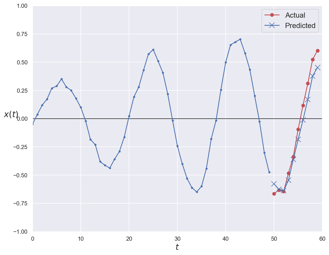
Multi-step forecasting

To forecast \(n\) timesteps ahead, we train the network to predict all \(n\) next values at once.

To do so, we need to turn the targets into vectors containing the next \(n\) values.

n_steps = 50
# Generate time series of length = n_steps + 10
series = generate_time_series(10000, n_steps + 10)

# Training inputs stay the same
# Targets are now the first (and only) feature for the last 10 time steps
x_train, y_train = series[:7000, :n_steps], series[:7000, -10:, 0]
x_val, y_val = series[7000:9000, :n_steps], series[7000:9000, -10:, 0]
x_test, y_test = series[9000:, :n_steps], series[9000:, -10:, 0]

print(f"series: {series.shape}")
print(f"x_train: {x_train.shape}, y_train: {y_train.shape}")
print(f"x_val: {x_val.shape}, y_val: {y_val.shape}")
print(f"x_test: {x_test.shape}, y_test: {y_test.shape}")

series: (10000, 60, 1)
x_train: (7000, 50, 1), y_train: (7000, 10)
x_val: (2000, 50, 1), y_val: (2000, 10)
x_test: (1000, 50, 1), y_test: (1000, 10)

multistep_rnn_model = Sequential()

multistep_rnn_model.add(SimpleRNN(units=20, return_sequences=True, input_shape=(None, 1)))
multistep_rnn_model.add(SimpleRNN(units=20))
# Predict 10 steps ahead
multistep_rnn_model.add(Dense(units=10))

multistep_rnn_model.summary()

Model: "sequential_2"
_________________________________________________________________
Layer (type)                 Output Shape              Param #   
=================================================================
simple_rnn_3 (SimpleRNN)     (None, None, 20)          440       
_________________________________________________________________
simple_rnn_4 (SimpleRNN)     (None, 20)                820       
_________________________________________________________________
dense_1 (Dense)              (None, 10)                210       
=================================================================
Total params: 1,470
Trainable params: 1,470
Non-trainable params: 0
_________________________________________________________________

# Compile and train the model

multistep_rnn_model.compile(optimizer="adam", loss="mse")

history = multistep_rnn_model.fit(
    x_train, y_train, epochs=15, verbose=0, validation_data=(x_val, y_val)
)

plot_loss(history)

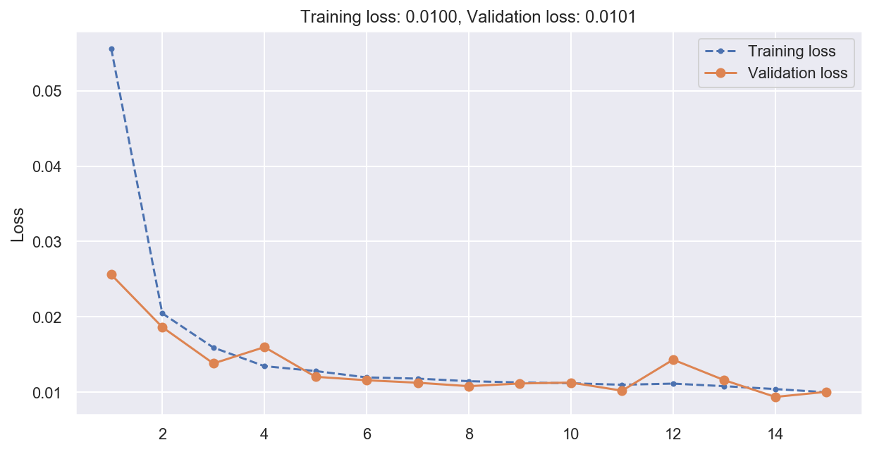
# Compute predictions and error on validation data

y_pred_multistep = multistep_rnn_model.predict(x_val)

print(f"Multistep RNN MSE: {np.mean(mean_squared_error(y_val, y_pred_multistep)):0.05f}")

Multistep RNN MSE: 0.01007

# Plot first validation series with ground truth and prediction
plot_series(
    series=x_val[0, :, 0], y_true=y_val[0], y_pred=y_pred_multistep[0]
)
plt.show()

LSTM, GRU and 1D convolutions

The limits of recurrent neurons

Basic RNN architectures suffer from a short-term memory problem. Because of data transformations when traversing the layers, some information is lost at each time step. Thus, they struggle to handle long-term dependencies between sequence elements.

Newer, more sophisticated RNN cell types like LSTM and GRU alleviate this limit.

LSTM cells

Long Short-Term Memory cells are a special kind of RNN cells, capable of learning long-term dependencies in input data. They were introduced in 1997 (original paper) and have been refined over the years.

An LSTM cell has a complex internal structure that make it able to:

• learn to recognize an important input,

• store it in the long-term state,

• preserve it for as long as it is needed,

• extract it whenever it is needed.

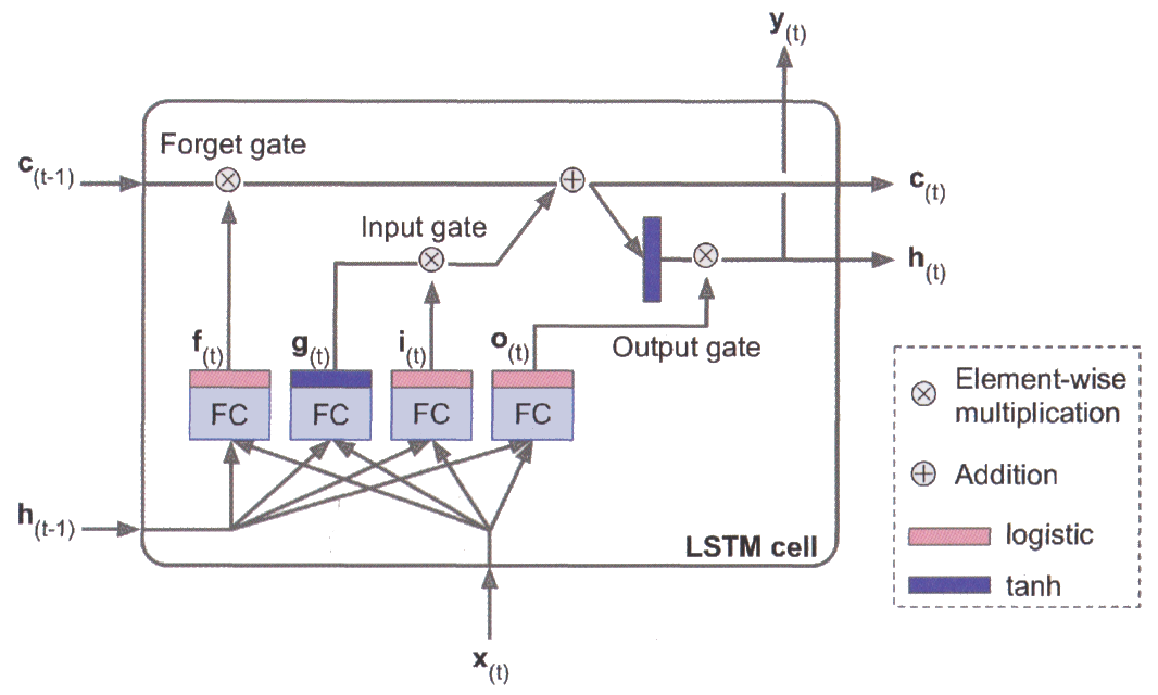
The cell’s state is split between \(\mathbf{h}_{(t)}\) (short-term state) and \(\mathbf{c}_{(t)}\) (long-term state).

• The layer that outputs \(\pmb{g}_{(t)}\) is the main layer. In a basic RNN layer, there would be nothing else.

• The forget gate (controlled by \(\pmb{f}_{(t)}\)) controls which parts of the previous long-term state \(\mathbf{c}_{(t-1)}\) should be erased.

• The input gate (controlled by \(\pmb{i}_{(t)}\)) controls which part of the main layer output should ne added to the long-term state.

• The output gate (controlled by \(\pmb{o}_{(t)}\)) controls which parts of the long-term state should be outputted at this time step.

Sigmoid-based layers output values near either 0 (gate closed) or 1 (gate open).

For more details, consult this step-by-step LSTM walkthrough.

# Build the simplest possible LSTM model
basic_lstm_model = Sequential()

# The LSTM layer's API is similar to the SimpleRNN's
basic_lstm_model.add(LSTM(units=1, input_shape=(None, 1)))

# 4 weights for input + 4 bias + 4 weights for short-term state = 12 parameters
basic_lstm_model.summary()

Model: "sequential_3"
_________________________________________________________________
Layer (type)                 Output Shape              Param #   
=================================================================
lstm (LSTM)                  (None, 1)                 12        
=================================================================
Total params: 12
Trainable params: 12
Non-trainable params: 0
_________________________________________________________________

# Build a LSTM-based model for time series forecasting
lstm_model = Sequential()

lstm_model.add(LSTM(units=20, return_sequences=True, input_shape=(None, 1)))
lstm_model.add(LSTM(units=20))
# Predict 10 steps ahead
lstm_model.add(Dense(units=10))

# First LSTM layer: 20x4 (input) + 20x4 (bias) + 20x20x4 (short-term state) = 1760
# Second LSTM layer: 20x20x4 (input) + 20x4 (bias) + 20x20x4 (short-term state) = 3280
# Dense layer: 10x20 (input) + 10 (bias) = 210
lstm_model.summary()

Model: "sequential_4"
_________________________________________________________________
Layer (type)                 Output Shape              Param #   
=================================================================
lstm_1 (LSTM)                (None, None, 20)          1760      
_________________________________________________________________
lstm_2 (LSTM)                (None, 20)                3280      
_________________________________________________________________
dense_2 (Dense)              (None, 10)                210       
=================================================================
Total params: 5,250
Trainable params: 5,250
Non-trainable params: 0
_________________________________________________________________

# Compile and train the model

lstm_model.compile(optimizer="adam", loss="mse")

history = lstm_model.fit(
    x_train, y_train, epochs=15, verbose=0, validation_data=(x_val, y_val)
)

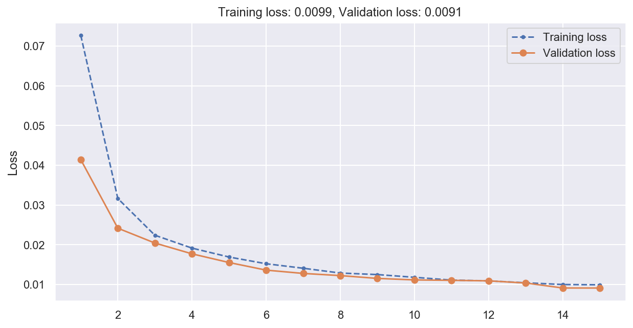
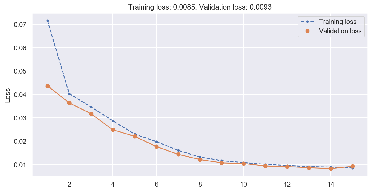
plot_loss(history)

# Compute predictions and error on validation data

y_pred_lstm = lstm_model.predict(x_val)

print(f"Multistep RNN MSE: {np.mean(mean_squared_error(y_val, y_pred_lstm)):0.05f}")

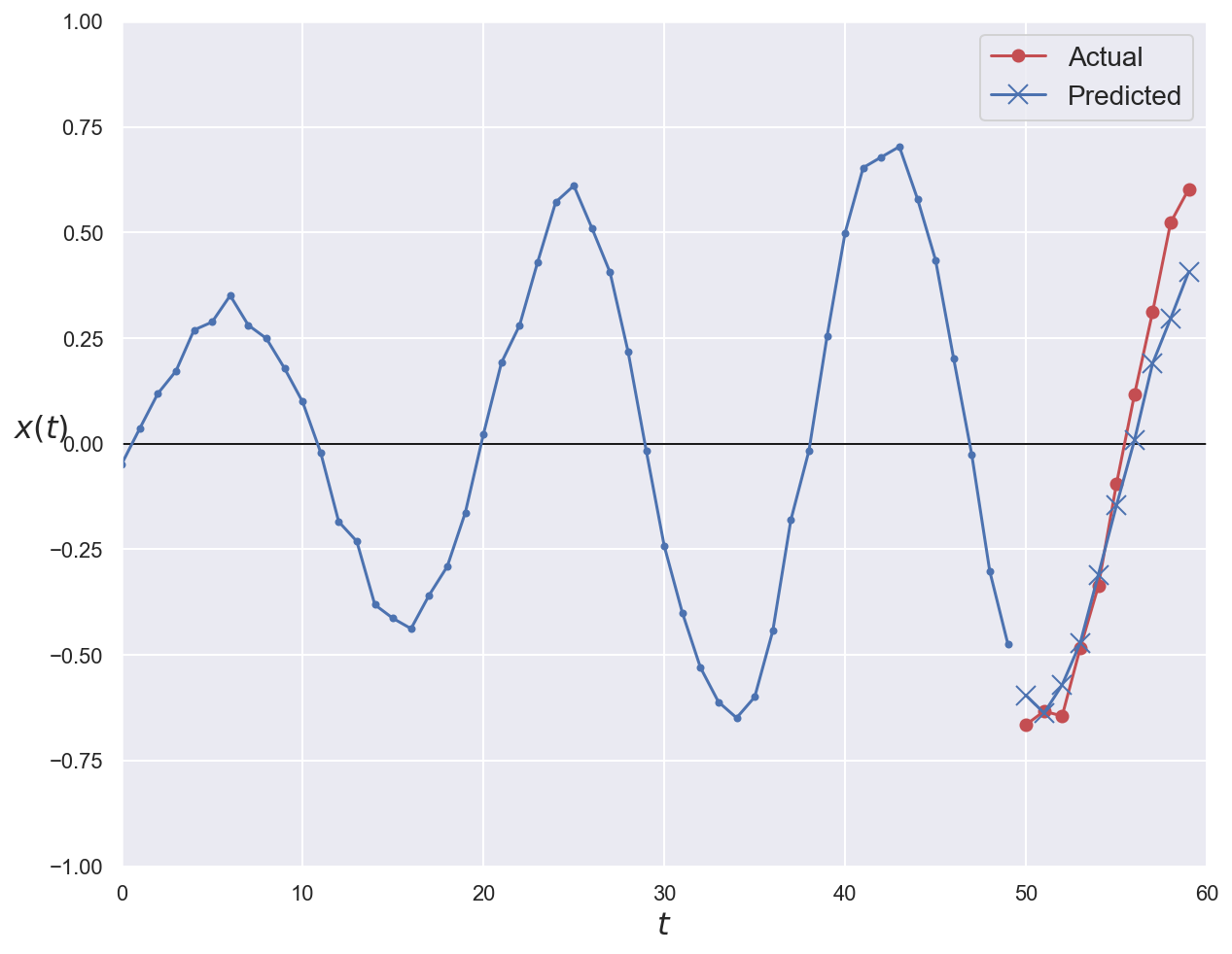
Multistep RNN MSE: 0.00911

# Plot first validation series with ground truth and prediction
plot_series(
    series=x_val[0, :, 0], y_true=y_val[0], y_pred=y_pred_lstm[0]
)
plt.show()

GRU cells

The Gated Recurrent Unit cell was introduced in 2014 (original paper).

It is a simplification of the LSTM cell that performs similarly well while being faster to train.

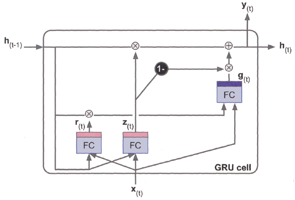
• Short- and long-time states are merged into the \(\mathbf{h}_{(t)}\) vector.

• A single update gate controller \(\pmb{z}_{(t)}\) manages both the forget and input gates. Whenever one is open, the other is closed.

• There is no output gate. However, the reset gate \(\pmb{r}_{(t)}\) controls which part of the previous state is shown to the main layer \(\pmb{g}_{(t)}\).

# Build the simplest possible GRU model
basic_gru_model = Sequential()

# The GRU layer's API is similar to the SimpleRNN's
basic_gru_model.add(GRU(units=1, input_shape=(None, 1)))

# Since TF 2.x, Keras separates biases for input and recurrent kernels
# 3 weights for input + 3 input bias + 3 weights for previous state + 3 state bias = 12
basic_gru_model.summary()

Model: "sequential_8"
_________________________________________________________________
Layer (type)                 Output Shape              Param #   
=================================================================
gru_5 (GRU)                  (None, 1)                 12        
=================================================================
Total params: 12
Trainable params: 12
Non-trainable params: 0
_________________________________________________________________

# Build a GRU-based model for time series forcasting
gru_model = Sequential()

gru_model.add(GRU(20, return_sequences=True, input_shape=(None, 1)))
gru_model.add(GRU(20))
# Predict 10 steps ahead
gru_model.add(Dense(10))

# First GRU layer: 20x3 (input) + 20x3 (input bias) + 20x20x3 (previous state) + 20x3 (state bias) = 1380
# Second GRU layer: 20x20x3 (input) + 20x3 (input bias) + 20x20x3 (previous state) + 20x3 (state bias) = 2520
# Dense layer: 10x20 (input) + 10 (bias) = 210
gru_model.summary()

Model: "sequential_6"
_________________________________________________________________
Layer (type)                 Output Shape              Param #   
=================================================================
gru_1 (GRU)                  (None, None, 20)          1380      
_________________________________________________________________
gru_2 (GRU)                  (None, 20)                2520      
_________________________________________________________________
dense_3 (Dense)              (None, 10)                210       
=================================================================
Total params: 4,110
Trainable params: 4,110
Non-trainable params: 0
_________________________________________________________________

# Compile and train the model

gru_model.compile(optimizer="adam", loss="mse")

history = gru_model.fit(
    x_train, y_train, epochs=15, verbose=0, validation_data=(x_val, y_val)
)

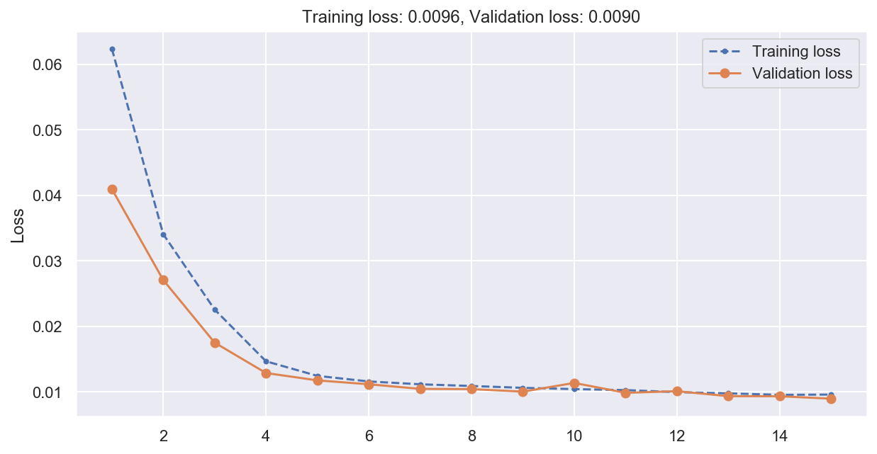
plot_loss(history)

# Compute predictions and error on validation data

y_pred_gru = gru_model.predict(x_val)

print(f"Multistep RNN MSE: {np.mean(mean_squared_error(y_val, y_pred_gru)):0.05f}")

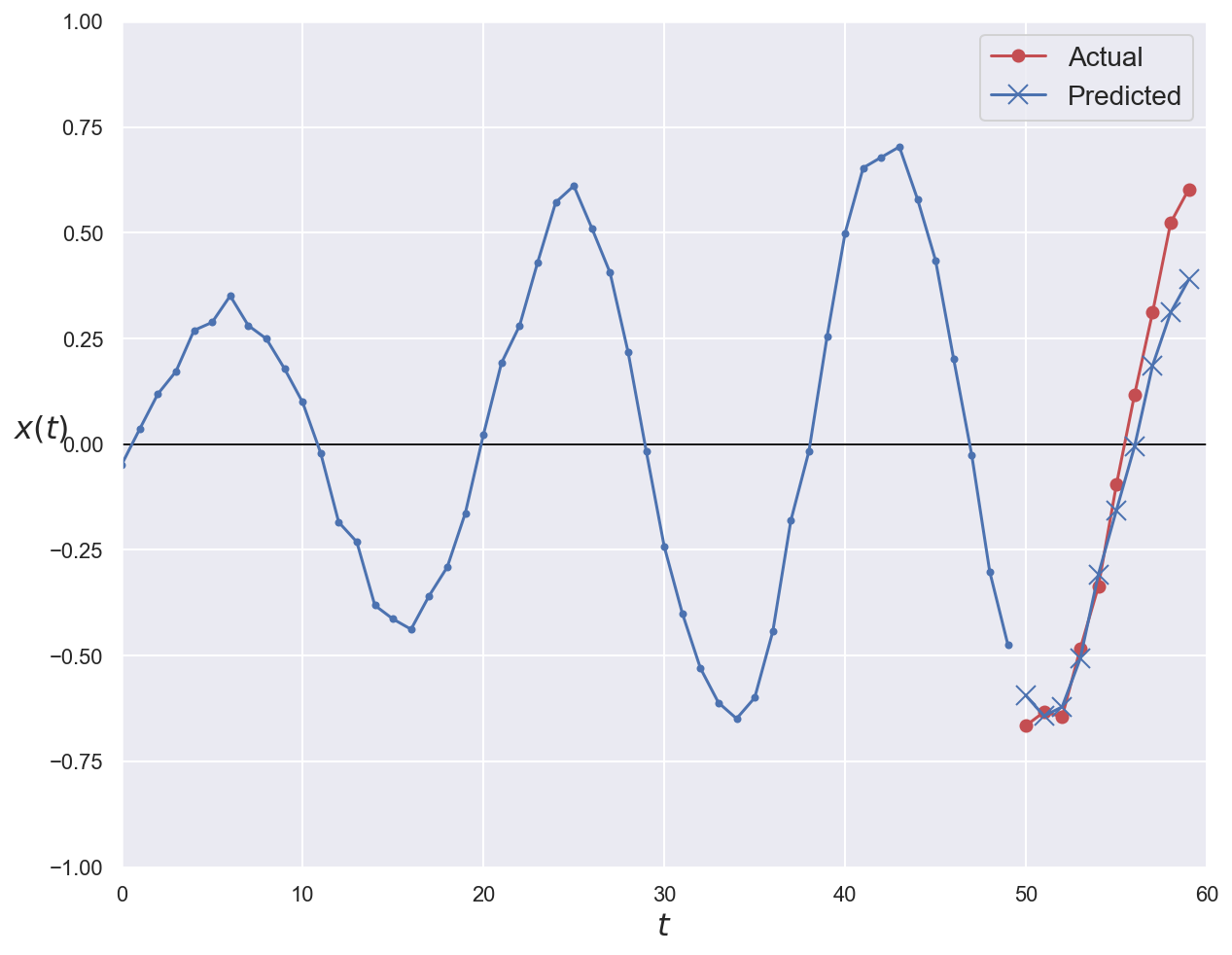
Multistep RNN MSE: 0.00926

# Plot first validation series with ground truth and prediction
plot_series(
    series=x_val[0, :, 0], y_true=y_val[0], y_pred=y_pred_gru[0]
)
plt.show()

Sequence processing with 1D convolutions

Despite their many qualities, LSTM and GRU cells still have a fairly limited short-term memory. To facilitate long-pattern detection in sequences of 100 time steps or more, a solution is to shorten the sequences by using 1D convolutions.

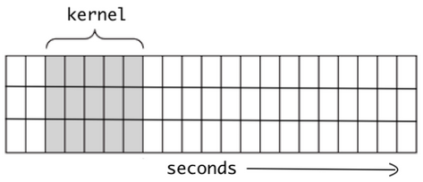
They work by treating time as a spatial dimension, and sliding several kernels across a sequence. Depending on the kernel size and stride (sliding step), the output sequence is typically shorter than the input one. 1D convolution will also detect higher-level features in the sequence, facilitating the work of subsequent layers.

# Create a model combining CNN and RNN operations
conv1d_gru_model = Sequential()

# Add a 1D convolution layer with 20 kernels of size 4
conv1d_gru_model.add(
    Conv1D(filters=20, kernel_size=4, strides=2, padding="valid", input_shape=(None, 1))
)
conv1d_gru_model.add(GRU(20, return_sequences=True))
conv1d_gru_model.add(GRU(20))
# Predict 10 steps ahead
conv1d_gru_model.add(Dense(10))

# Conv1D layer: 20x4 (kernels weights) + 20 (kernels bias) = 100
# GRU layers: 20x20x3 (input) + 20x3 (input bias) + 20x20x3 (previous state) + 20x3 (state bias) = 2520
# Dense layer: 10x20 (input) + 10 (bias) = 210
conv1d_gru_model.summary()

Model: "sequential_7"
_________________________________________________________________
Layer (type)                 Output Shape              Param #   
=================================================================
conv1d (Conv1D)              (None, None, 20)          100       
_________________________________________________________________
gru_3 (GRU)                  (None, None, 20)          2520      
_________________________________________________________________
gru_4 (GRU)                  (None, 20)                2520      
_________________________________________________________________
dense_4 (Dense)              (None, 10)                210       
=================================================================
Total params: 5,350
Trainable params: 5,350
Non-trainable params: 0
_________________________________________________________________

# Compile and train the model

conv1d_gru_model.compile(optimizer="adam", loss="mse")

history = conv1d_gru_model.fit(
    x_train, y_train, epochs=15, verbose=0, validation_data=(x_val, y_val)
)

plot_loss(history)

# Compute predictions and error on validation data

y_pred_conv1d_gru = conv1d_gru_model.predict(x_val)

print(f"Multistep RNN MSE: {np.mean(mean_squared_error(y_val, y_pred_conv1d_gru)):0.05f}")

Multistep RNN MSE: 0.00898

# Plot first validation series with ground truth and prediction
plot_series(
    series=x_val[0, :, 0], y_true=y_val[0], y_pred=y_pred_conv1d_gru[0]
)
plt.show()