Decision Trees & Random Forests

Decision Trees & Random Forests#

Environment setup#

import platform

print(f"Python version: {platform.python_version()}")
assert platform.python_version_tuple() >= ("3", "6")

import numpy as np
import matplotlib.pyplot as plt
from matplotlib.colors import ListedColormap
import seaborn as sns
import pandas as pd
import graphviz

Python version: 3.7.5

# Setup plots
%matplotlib inline
plt.rcParams["figure.figsize"] = 10, 8
%config InlineBackend.figure_format = 'retina'
sns.set()

import sklearn

print(f"scikit-learn version: {sklearn.__version__}")

from sklearn.datasets import load_iris
from sklearn.tree import (
    DecisionTreeClassifier,
    DecisionTreeRegressor,
    plot_tree,
    export_graphviz,
)
from sklearn.ensemble import RandomForestClassifier
from sklearn.model_selection import cross_val_score

scikit-learn version: 0.22.1

Decision Trees#

(Heavily inspired by Chapter 6 of Hands-On Machine Learning by Aurélien Géron)

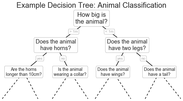
Decision Trees in a nutshell#

Supervised method, used for classification or regression.
Build a tree-like structure based on a series of questions on the data.

Example: training a Decision Tree to classify flowers#

Iris is a well-known multiclass dataset. It contains 3 classes of flowers with 50 samples each. There are a total of 4 features for each sample:

sepal length
sepal width
petal length
petal width

# Load the Iris dataset
iris = load_iris()

# Put it into a DataFrame for visualization purposes
df_iris = pd.DataFrame(iris.data, columns=iris.feature_names)
# Add target and class columns to DataFrame
df_iris["target"] = iris.target
df_iris["class"] = iris.target_names[iris.target]
# Show 10 random samples
df_iris.sample(n=10)

	sepal length (cm)	sepal width (cm)	petal length (cm)	petal width (cm)	target	class
145	6.7	3.0	5.2	2.3	2	virginica
80	5.5	2.4	3.8	1.1	1	versicolor
113	5.7	2.5	5.0	2.0	2	virginica
120	6.9	3.2	5.7	2.3	2	virginica
126	6.2	2.8	4.8	1.8	2	virginica
96	5.7	2.9	4.2	1.3	1	versicolor
38	4.4	3.0	1.3	0.2	0	setosa
81	5.5	2.4	3.7	1.0	1	versicolor
88	5.6	3.0	4.1	1.3	1	versicolor
0	5.1	3.5	1.4	0.2	0	setosa

# Use only last two features (petal length and width)
# Thus, we can plot a 2D decision boundary

x_train_2feat = iris.data[:, 2:]
y_train_2feat = iris.target

print(f"x_train: {x_train_2feat.shape}")
print(f"y_train: {y_train_2feat.shape}")

x_train: (150, 2)
y_train: (150,)

# Train a DT on the simplified dataset
dt_model = DecisionTreeClassifier(max_depth=2, random_state=42)
dt_model.fit(x_train_2feat, y_train_2feat)

# Compute accuracy on training set
acc = dt_model.score(x_train_2feat, y_train_2feat)
print(f"Training accuracy: {acc:.5f}")

Training accuracy: 0.96000

# Plot the DT
# If using Jupyter locally, install graphviz with this command: conda install python-graphviz
dot_data = export_graphviz(
    dt_model,
    out_file=None,
    feature_names=iris.feature_names[2:],
    class_names=iris.target_names,
    filled=True,
    rounded=True,
    special_characters=True,
)
graphviz.Source(dot_data)

../_images/88898803432a655361acb544147d86cdacb00a00fd3cdb599a48da249ddd60cf.svg

Tree nodes#

Each node is a step in the decision process, starting with the root node (depth 0). Leaf nodes represent predictions of the model.

Node attributes are:

Gini: measure of the node impurity.
Samples: number of samples the node applies to.
Value: number of samples of each class the node applies to.

The Gini score#

\(G_i = 1- \sum_{k=1}^K {p_{i, k}}^2\)
\(p_{i, k}\): ratio of class k instances in the \(i^{th}\) node.
\(Gini = 0\): all samples it applies to belong to the same class (“pure” node).

Other possible measure: entropy (level of disorder).

Example: Gini scores for the trained Decision Tree#

Root node:

\[G_0 = 1 - ((\frac{50}{150})^2 + (\frac{50}{150})^2 + (\frac{50}{150})^2) = 1 - (\frac{1}{9} + \frac{1}{9} + \frac{1}{9}) = \frac{2}{3}\]

Depth 1, left node:

\[G_1 = 1 - ((\frac{50}{50})^2 + (\frac{0}{50})^2 + (\frac{0}{50})^2) = 1 - (1 + 0 + 0) = 0\]

Depth 2, left node:

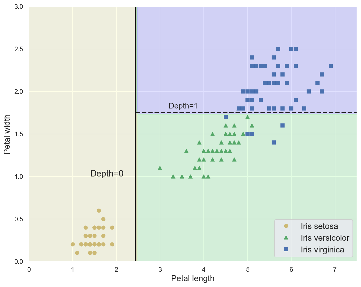
\[G_3 = 1 - ((\frac{0}{54})^2 + (\frac{49}{54})^2 + (\frac{5}{54})^2) \simeq 0.168\]

Example: decision boundaries for the trained Decision Tree#

plot_iris_decision_boundary(dt_model, x_train_2feat, y_train_2feat)
# Plot separation lines
plt.plot([2.45, 2.45], [0, 3], "k-", linewidth=2)
plt.plot([2.45, 7.5], [1.75, 1.75], "k--", linewidth=2)
plt.text(1.40, 1.0, "Depth=0", fontsize=15)
plt.text(3.2, 1.80, "Depth=1", fontsize=13)
plt.show()

../_images/09be75fa5b9f47c21027031d6768c0ef9a3fd5ab4a0c69071a500c89d8152d2b.png

Using a Decision Tree for predictions#

Using the new sample data, the tree is traversed to find the leaf node for that sample.
Class probabilities are the ratios of samples of each class for this node.

# Define some new flower data
x_new = [[5, 1.5]]

# Print predicted class probabilities
# 0/54 for "setosa", 49/54 for "versicolor", 5/54 for "virginica"
print(dt_model.predict_proba(x_new))

# Print predicted class
print(iris.target_names[dt_model.predict(x_new)])

[[0.         0.90740741 0.09259259]]
['versicolor']

The training process#

The CART (Classification And Regression Tree) algorithm creates binary trees.

At each depth, it looks for the highest Gini gain by finding the feature and the threshold that produces the purest subsets (weighted by their size). Then, its splits the subsets recursively according to the same logic.

It stops once no split will further reduce impurity, or when it reaches the maximum depth.

Example: training a Decision Tree on planar data#

Three classes with 3 samples each, two features \(x\) and \(y\).

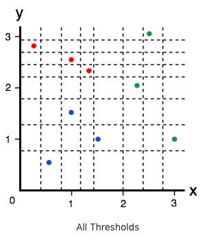
\(G_{initial} = 1 - ((\frac{3}{9})^2 + (\frac{3}{9})^2 + (\frac{3}{9})^2) = \frac{2}{3}\)

Impurity gain with \(x=0.4\):

\(G_{left|x=0.4} = 1 - ((\frac{1}{1})^2 + (\frac{0}{1})^2 + (\frac{0}{1})^2) = 0\;\;G_{right|x=0.4} = 1 - ((\frac{2}{8})^2 + (\frac{3}{8})^2 + (\frac{3}{8})^2) = \frac{21}{32}\)
\(Gain_{x=0.4} = G_{initial} - (\frac{1}{9}G_{left|x=0.4} + \frac{8}{9}G_{right|x=0.4}) = \frac{2}{3} - \frac{7}{12} = \frac{1}{12}\)

Impurity gain with \(x=2\):

\(G_{left|x=2} = 1 - ((\frac{3}{6})^2 + (\frac{3}{6})^2 + (\frac{0}{6})^2) = 0,5\;\;G_{right|x=2} = 1 - ((\frac{0}{3})^2 + (\frac{0}{3})^2 + (\frac{3}{3})^2) = 0\)
\(Gain_{x=2} = G_{initial} - (\frac{6}{9}G_{left|x=2} + \frac{3}{9}G_{right|x=2}) = \frac{2}{3} - \frac{1}{3} = \frac{1}{3}\)

Decision Trees for regression problems#

Decision Tree can also perform regression tasks.

Instead of predicting a class, it outputs a value which is the average of all training samples associated with the leaf node reached during traversal.

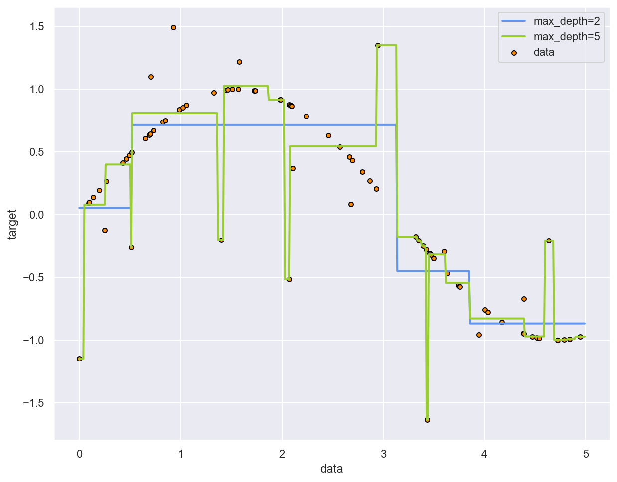
Example: fitting a sine curve with a Decision Tree#

# Taken from https://scikit-learn.org/stable/auto_examples/tree/plot_tree_regression.html
# Create a random dataset
rng = np.random.RandomState(1)
x_sin = np.sort(5 * rng.rand(80, 1), axis=0)
y_sin = np.sin(x_sin).ravel()
y_sin[::5] += 3 * (0.5 - rng.rand(16))

# Fit regression DT
dt_reg_model1 = DecisionTreeRegressor(max_depth=2)
dt_reg_model1.fit(x_sin, y_sin)

DecisionTreeRegressor(ccp_alpha=0.0, criterion='mse', max_depth=2,
                      max_features=None, max_leaf_nodes=None,
                      min_impurity_decrease=0.0, min_impurity_split=None,
                      min_samples_leaf=1, min_samples_split=2,
                      min_weight_fraction_leaf=0.0, presort='deprecated',
                      random_state=None, splitter='best')

# Plot the DT
# If using Jupyter locally, install graphviz with this command: conda install python-graphviz
dot_data = export_graphviz(
    dt_reg_model1,
    out_file=None,
    feature_names=["x"],
    filled=True,
    rounded=True,
    special_characters=True,
)
graphviz.Source(dot_data)

../_images/425013ac23779a6a48d751241b2a6b09f18f1676a6f38da8151ceb31cd1c5278.svg

# Train another regression DT on same dataset
dt_reg_model2 = DecisionTreeRegressor(max_depth=5)
dt_reg_model2.fit(x_sin, y_sin)

# Predict values for both DT
x_test = np.arange(0.0, 5.0, 0.01)[:, np.newaxis]
y_pred_1 = dt_reg_model1.predict(x_test)
y_pred_2 = dt_reg_model2.predict(x_test)

# Plot the results
plt.figure()
plt.scatter(x_sin, y_sin, s=20, edgecolor="black", c="darkorange", label="data")
plt.plot(x_test, y_pred_1, color="cornflowerblue", label="max_depth=2", linewidth=2)
plt.plot(x_test, y_pred_2, color="yellowgreen", label="max_depth=5", linewidth=2)
plt.xlabel("data")
plt.ylabel("target")
plt.legend()
plt.show()

../_images/c849a04333a0b0b59940b01dd070a25af4217a3f04b0558634244cf6f6b4f558.png

Advantages of Decision Trees#

Versatility
Very fast inference
Intuitive and interpretable (white box)
No feature scaling or encoding required

Decision Trees shortcomings#

Main problem: overfitting. Regularization is possible through hyperparameters:
- Maximum depth of the tree.
- Minimum number of samples needed to split a node.
- Minimum number of samples for any leaf node.
- Maximum number of leaf nodes.
Sensibility to small variations in the training data.

Ensemble learning#

(Heavily inspired by Chapter 7 of Hands-On Machine Learning by Aurélien Géron)

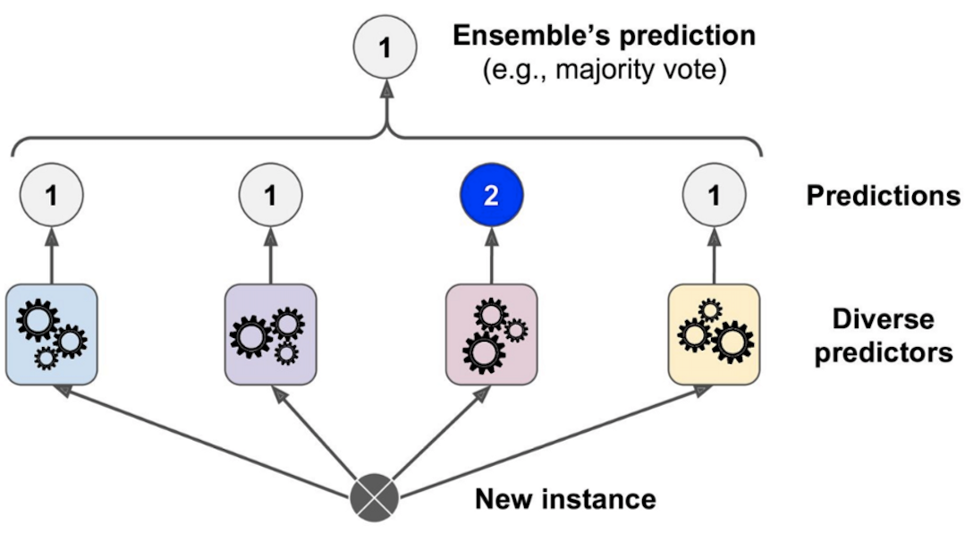
General idea#

Combining several predictors will lead to better results.
A group of predictors is called an ensemble.
Works best when predictors are diverse.
Less interpretable and harder to tune than an individual predictor.

Hard voting classifiers#

Soft voting classifiers#

Use class probabilities rather than class predictions.
Often yields better results than hard voting (highly confident predictions have more weight).

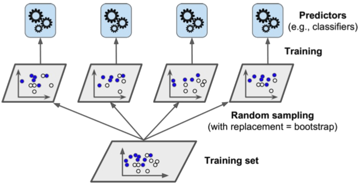
Bagging and pasting#

Both methods train several predictors with the same algorithm on different random samples of the training set. The ensemble’s result is computed by aggregating (i.e. most frequent or average) the predictions of individual predictors.

Only bagging (bootstrap aggregating) allows samples to be repeated for the same predictor.

Boosting#

Bagging and pasting methods rely on the simultaneous construction of several independent predictors.

On the contrary, boosting methods train predictors sequentially, each one trying to correct its predecessor.

AdaBoost#

The core principle of AdaBoost (Adaptative Boosting) is to train several predictors on repeatedly modified versions of the dataset. The weights of incorrectly predicted instances are adjusted such that subsequent predictors focus more on difficult cases.

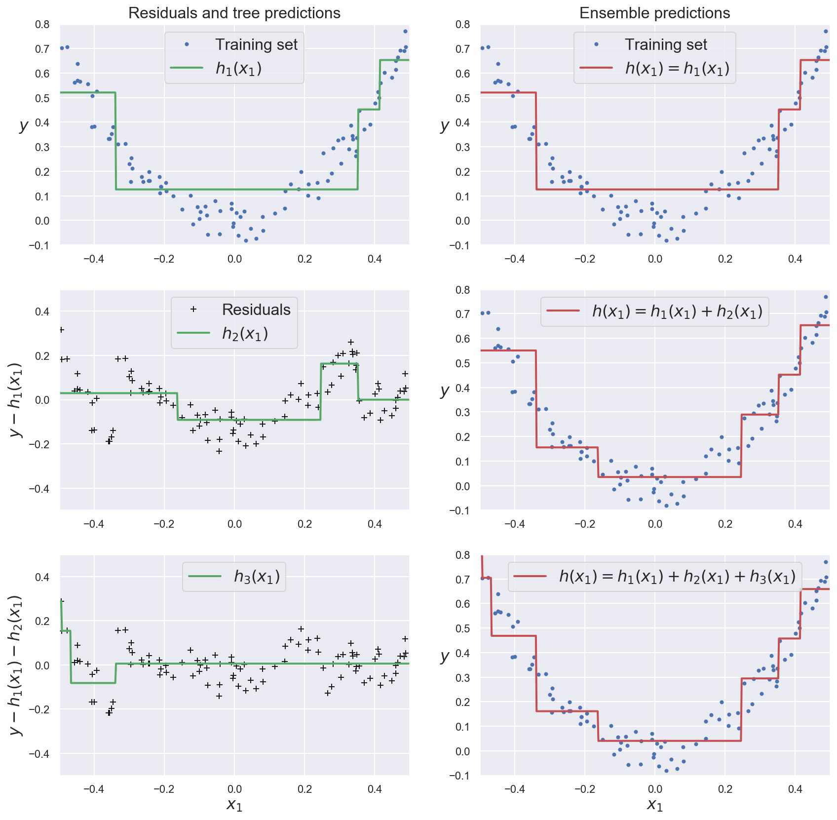
Gradient boosting#

This methods train subsequent predictors on the residual errors made by the previous ones.

The ensemble’s prediction is the sum of all individual predictions.

Example: gradient boosting for regression#

def noisy_quadratic(x):
    return 3 * x[:, 0] ** 2 + 0.05 * np.random.randn(len(x))

# Generate a noisy quadratic dataset
x_boost = np.random.rand(100, 1) - 0.5
y_boost = noisy_quadratic(x_boost)


def grow_regression_tree(x, y):
    """Create and train a Decision Tree Regressor"""
    dtr_model = DecisionTreeRegressor(max_depth=2, random_state=42)
    dtr_model.fit(x, y)
    return dtr_model

# Train a DTR on initial dataset
dtr_model_1 = grow_regression_tree(x_boost, y_boost)
error_1 = y_boost - dtr_model_1.predict(x_boost)

# Train another DTR to predict the residual error of first DTR
dtr_model_2 = grow_regression_tree(x_boost, error_1)
error_2 = error_1 - dtr_model_2.predict(x_boost)

# Train another DTR to predict the residual error of second DTR
dtr_model_3 = grow_regression_tree(x_boost, error_2)
error_3 = error_2 - dtr_model_2.predict(x_boost)

# Generate test input and target
x_test = np.array([[0.05]])
y_test = noisy_quadratic(x_test)

# Compute error of first predictor
y_pred_1 = dtr_model_1.predict(x_test)
print(f"First DTR error: {abs(y_test - y_pred_1)}")

# Compute error of boosted ensemble
y_pred_ens = sum(dtr_model.predict(x_test) for dtr_model in (dtr_model_1, dtr_model_2, dtr_model_3))
print(f"Boosted ensemble error: {abs(y_test - y_pred_ens)}")

First DTR error: [0.1301599]
Boosted ensemble error: [0.04451791]

../_images/682fe4904d71c8db16e212da93be72327e02a44a37729366c65acecf1767d165.png

Random Forests#

Random Forests in a nutshell#

Ensemble of Decision Trees, generally trained via bagging.
May be used for classification or regression.
Trees are grown using a random subset of features.
Ensembling mitigates the individual shortcomings of Decision Trees (overfitting, sensibility to small changes in the dataset).
On the other hand, results are less interpretable.

Example: training a Random Forest to classify flowers#

# Use whole Iris dataset
x_train = iris.data
y_train = iris.target

# Create a Random Forest classifier
# n_estimators: number of predictors (Decision Trees)
rf_model = RandomForestClassifier(n_estimators=200)

# Train the RF on the dataset
rf_model.fit(x_train, y_train)

# Compute cross-validation scores for the RF
scores = cross_val_score(rf_model, x_train, y_train, cv=5)

cv_acc = scores.mean()
print(f"Mean CV accuracy: {cv_acc:.05f}")

Mean CV accuracy: 0.96000