Linear Regression

Linear Regression#

Environment setup#

import platform

print(f"Python version: {platform.python_version()}")
assert platform.python_version_tuple() >= ("3", "6")

import numpy as np
import matplotlib.pyplot as plt
import seaborn as sns
import plotly
import plotly.graph_objs as go
import pandas as pd

print(f"NumPy version: {np.__version__}")

Python version: 3.7.5
NumPy version: 1.18.1

# Setup plots
%matplotlib inline
plt.rcParams["figure.figsize"] = 10, 8
%config InlineBackend.figure_format = "retina"
sns.set()

# Configure Plotly to be rendered inline in the notebook.
plotly.offline.init_notebook_mode()

import sklearn

print(f"scikit-learn version: {sklearn.__version__}")
assert sklearn.__version__ >= "0.20"

from sklearn.model_selection import train_test_split
from sklearn.linear_model import LinearRegression, SGDRegressor, Ridge
from sklearn.metrics import mean_squared_error
from sklearn.preprocessing import PolynomialFeatures, StandardScaler
from sklearn.pipeline import Pipeline

scikit-learn version: 0.22.1

Introduction#

Linear regression in a nutshell#

A linear regression model searches for a linear relationship between inputs (features) and output (target).

Problem formulation#

A linear model makes a prediction by computing a weighted sum of the input features, plus a constant term called bias (or sometimes intercept).

\[y' = \theta_0 + \theta_1x_1 + \dotsc + \theta_nx_n\]

\(y'\) is the model’s output (prediction).
\(n\) is the number of features for a data sample.
\(x_i, i \in [1..n]\) is the value of the \(i\)th feature.
\(\theta_i, i \in [0..n]\) is \(i\)th model parameter. \(\theta_0\) is the bias term.

The goal is to find the best set of parameters.

Example: using a linear model to predict country happiness#

(Inspired by Homemade Machine Learning by Oleksii Trekhleb)

The World Happiness Report ranks 155 countries by their happiness levels. Several economic and social indicators (GDP, degree of freedom, level of corruption…) are recorded for each country.

Can a linear model accurately predict country happiness based on these indicators ?

Data loading and analysis#

# Load World Happiness Report for 2017
dataset_url = "https://raw.githubusercontent.com/bpesquet/mlhandbook/master/_datasets/world-happiness-report-2017.csv"
df_happiness = pd.read_csv(dataset_url)

# Print dataset shape (rows and columns)
print(f"Dataset shape: {df_happiness.shape}")

Dataset shape: (155, 12)

# Print a concise summary of the dataset
df_happiness.info()

<class 'pandas.core.frame.DataFrame'>
RangeIndex: 155 entries, 0 to 154
Data columns (total 12 columns):
 #   Column                         Non-Null Count  Dtype  
---  ------                         --------------  -----  
 0   Country                        155 non-null    object 
 1   Happiness.Rank                 155 non-null    int64  
 2   Happiness.Score                155 non-null    float64
 3   Whisker.high                   155 non-null    float64
 4   Whisker.low                    155 non-null    float64
 5   Economy..GDP.per.Capita.       155 non-null    float64
 6   Family                         155 non-null    float64
 7   Health..Life.Expectancy.       155 non-null    float64
 8   Freedom                        155 non-null    float64
 9   Generosity                     155 non-null    float64
 10  Trust..Government.Corruption.  155 non-null    float64
 11  Dystopia.Residual              155 non-null    float64
dtypes: float64(10), int64(1), object(1)
memory usage: 14.7+ KB

# Show the 10 first samples
df_happiness.head(n=10)

	Country	Happiness.Rank	Happiness.Score	Whisker.high	Whisker.low	Economy..GDP.per.Capita.	Family	Health..Life.Expectancy.	Freedom	Generosity	Trust..Government.Corruption.	Dystopia.Residual
0	Norway	1	7.537	7.594445	7.479556	1.616463	1.533524	0.796667	0.635423	0.362012	0.315964	2.277027
1	Denmark	2	7.522	7.581728	7.462272	1.482383	1.551122	0.792566	0.626007	0.355280	0.400770	2.313707
2	Iceland	3	7.504	7.622030	7.385970	1.480633	1.610574	0.833552	0.627163	0.475540	0.153527	2.322715
3	Switzerland	4	7.494	7.561772	7.426227	1.564980	1.516912	0.858131	0.620071	0.290549	0.367007	2.276716
4	Finland	5	7.469	7.527542	7.410458	1.443572	1.540247	0.809158	0.617951	0.245483	0.382612	2.430182
5	Netherlands	6	7.377	7.427426	7.326574	1.503945	1.428939	0.810696	0.585384	0.470490	0.282662	2.294804
6	Canada	7	7.316	7.384403	7.247597	1.479204	1.481349	0.834558	0.611101	0.435540	0.287372	2.187264
7	New Zealand	8	7.314	7.379510	7.248490	1.405706	1.548195	0.816760	0.614062	0.500005	0.382817	2.046456
8	Sweden	9	7.284	7.344095	7.223905	1.494387	1.478162	0.830875	0.612924	0.385399	0.384399	2.097538
9	Australia	10	7.284	7.356651	7.211349	1.484415	1.510042	0.843887	0.601607	0.477699	0.301184	2.065211

# Plot histograms for all numerical attributes
df_happiness.hist(bins=20, figsize=(16, 12))
plt.show()

../_images/bc5c9216a7e2b82de4cc1ca203901e585c864959bbd2a476befde48df1c08213.png

Univariate regression#

Only one feature is used by the model, which has two parameters.

\[y' = \theta_0 + \theta_1x\]

Example: predict country happiness using only GDP#

def filter_dataset(df_data, input_features, target_feature):
    """Return a dataset containing only the selected input and output features"""
    
    feature_list = input_features + [target_feature]
    return df_data[feature_list]

# Define GDP as sole input feature
input_features_uni = ["Economy..GDP.per.Capita."]
# Define country happiness as target
target_feature = "Happiness.Score"

df_happiness_uni = filter_dataset(df_happiness, input_features_uni, target_feature)

# Show 10 random samples
df_happiness_uni.sample(n=10)

	Economy..GDP.per.Capita.	Happiness.Score
89	0.982409	5.182
146	0.397249	3.591
121	0.792221	4.315
67	1.101803	5.525
97	0.596220	5.004
123	0.808964	4.291
32	1.433627	6.422
93	0.788548	5.074
26	1.343280	6.527
78	1.081166	5.273

Data splitting#

def split_dataset(df_data, input_features, target_feature):
    """Split dataset between training and test sets, keeping only selected features"""
    
    df_train, df_test = train_test_split(df_data, test_size=0.2)

    print(f"Training dataset: {df_train.shape}")
    print(f"Test dataset: {df_test.shape}")

    x_train = df_train[input_features].to_numpy()
    y_train = df_train[target_feature].to_numpy()

    x_test = df_test[input_features].to_numpy()
    y_test = df_test[target_feature].to_numpy()

    print(f"Training data: {x_train.shape}, labels: {y_train.shape}")
    print(f"Test data: {x_test.shape}, labels: {y_test.shape}")

    return x_train, y_train, x_test, y_test

x_train_uni, y_train_uni, x_test_uni, y_test_uni = split_dataset(
    df_happiness_uni, input_features_uni, target_feature
)

Training dataset: (124, 2)
Test dataset: (31, 2)
Training data: (124, 1), labels: (124,)
Test data: (31, 1), labels: (31,)

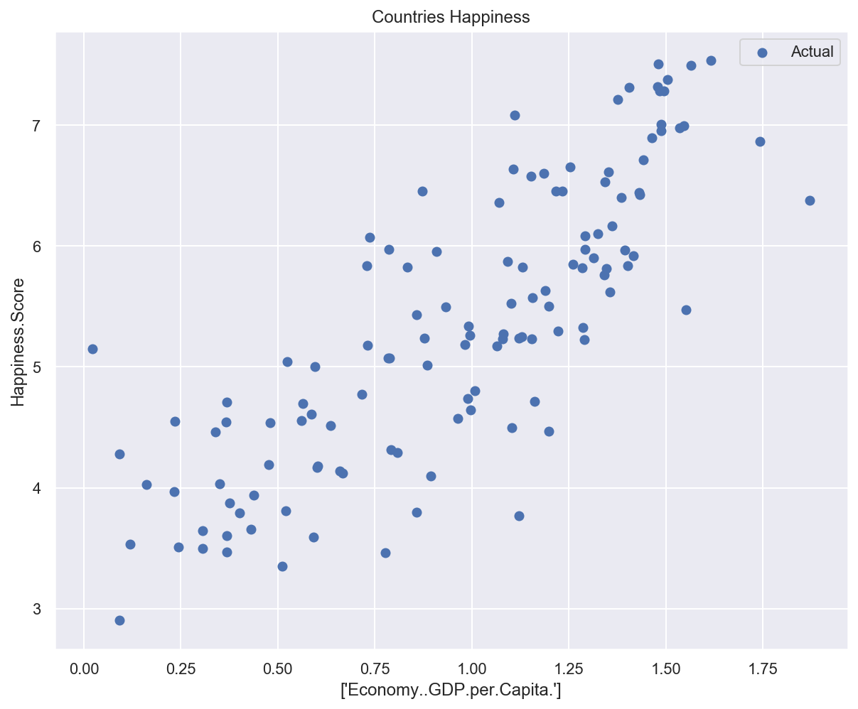
Data plotting#

# Plot training data
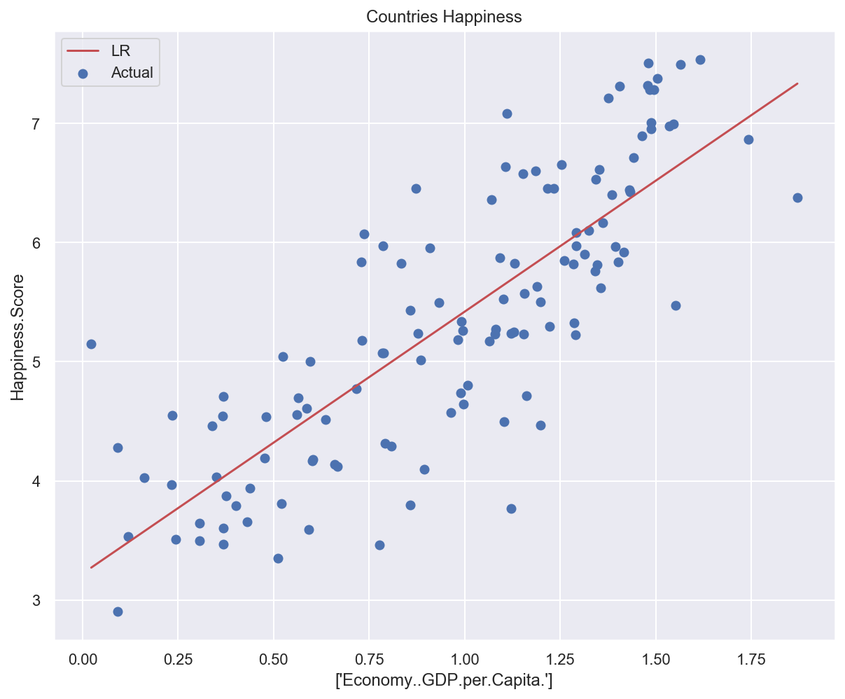
plot_univariate(x_train_uni, y_train_uni, input_features_uni, target_feature)

../_images/4a93933ed69f7ca135885a66b8586180a388bf440bc5b5bdb39234fba9e23014.png

Analytical approach: normal equation#

Problem formulation#

\(\pmb{x}^{(i)}\): \(i\)th data sample, vector of \(n+1\) features \(x^{(i)}_j\) with \(x^{(i)}_0 = 1\).
\(\pmb{\theta}\): parameters of the linear model, vector of \(n+1\) values \(\theta_j\).
\(\mathcal{h}_\theta\): hypothesis function (relationship between inputs and targets).
\(y'^{(i)}\): model output for the \(i\)th sample.

\[\begin{split}\pmb{x}^{(i)} = \begin{pmatrix} \ x^{(i)}_0 \\ \ x^{(i)}_1 \\ \ \vdots \\ \ x^{(i)}_n \end{pmatrix} \in \pmb{R}^{n+1} \;\;\; \pmb{\theta} = \begin{pmatrix} \ \theta_0 \\ \ \theta_1 \\ \ \vdots \\ \ \theta_n \end{pmatrix} \in \pmb{R}^{n+1}\end{split}\]

\[y'^{(i)} = \mathcal{h}_\theta(x^{(i)}) = \theta_0 + \theta_1x^{(i)}_1 + \dotsc + \theta_nx^{(i)}_n = \pmb{\theta}^T\pmb{x}^{(i)}\]

Loss function#

We use the Mean Squared Error (MSE). RMSE is also a possible choice.

\[\mathcal{L}(\pmb{\theta}) = \frac{1}{m}\sum_{i=1}^m (y'^{(i)} - y^{(i)})^2 = \frac{1}{m}\sum_{i=1}^m (\mathcal{h}_\theta(x^{(i)}) - y^{(i)})^2\]

Analytical solution#

Technique for computing the regression coefficients \(\theta_i\) analytically (by calculus).
One-step learning algorithm (no iterations).
Also called Ordinary Least Squares.

\[\pmb{\theta^{*}} = (\pmb{X}^T\pmb{X})^{-1}\pmb{X}^T\pmb{y}\]

\(\pmb{\theta^*}\) is the parameter vector that minimizes the loss function \(\mathcal{L}(\theta)\).
This result is called the Normal Equation.

Math proof (optional)#

(Inspired by Derivation of the Normal Equation for linear regression and ML From Scratch, Part 1: Linear Regression)

Vectorized notation#

\(\pmb{X}\): matrix of input data (design matrix). Each line corresponds to a sample.
\(\pmb{y}\): vector of target values.

\[\begin{split}\pmb{X} = \begin{bmatrix} \ x^{(0)T} \\ \ x^{(1)T} \\ \ \vdots \\ \ x^{(m)T} \\ \end{bmatrix} = \begin{bmatrix} \ x^{(1)}_0 & x^{(1)}_1 & \cdots & x^{(1)}_n \\ \ x^{(2)}_0 & x^{(2)}_1 & \cdots & x^{(2)}_n \\ \ \vdots & \vdots & \ddots & \vdots \\ \ x^{(m)}_0 & x^{(m)}_1 & \cdots & x^{(m)}_n \end{bmatrix}\;\;\; \pmb{y} = \begin{pmatrix} \ y^{(1)} \\ \ y^{(2)} \\ \ \vdots \\ \ y^{(m)} \end{pmatrix}\end{split}\]

\[\begin{split}\pmb{X}\pmb{\theta} = \begin{pmatrix} \ \theta_0 + \theta_1x^{(1)}_1 + \dotsc + \theta_nx^{(1)}_n \\ \ \theta_0 + \theta_1x^{(2)}_1 + \dotsc + \theta_nx^{(2)}_n \\ \ \vdots \\ \ \theta_0 + \theta_1x^{(m)}_1 + \dotsc + \theta_nx^{(m)}_n \end{pmatrix} = \begin{pmatrix} \ \mathcal{h}_\theta(x^{(1)}) \\ \ \mathcal{h}_\theta(x^{(2)}) \\ \ \vdots \\ \ \mathcal{h}_\theta(x^{(m)}) \end{pmatrix}\end{split}\]

Vectorized loss#

The loss can also be expressed using a vectorized notation.

\[\mathcal{L}(\theta) = \frac{1}{m}\sum_{i=1}^m (\mathcal{h}_\theta(x^{(i)}) - y^{(i)})^2 = \frac{1}{m}{{\lVert{\pmb{X}\pmb{\theta} - \pmb{y}}\rVert}_2}^2\]

The squared norm of a vector \(\pmb{v}\) is the inner product of that vector with its transpose: \(\sum_{i=1}^n v_i^2 = \pmb{v}^T \pmb{v}\).

\[\mathcal{L}(\theta) = \frac{1}{m}(\pmb{X}\pmb{\theta} - \pmb{y})^T(\pmb{X}\pmb{\theta} - \pmb{y})\]

The previous expression can be developped.

\[\mathcal{L}(\theta) = \frac{1}{m}\left((\pmb{X}\pmb{\theta})^T - \pmb{y}^T)(\pmb{X}\pmb{\theta} - \pmb{y}\right) = \frac{1}{m}\left((\pmb{X}\pmb{\theta})^T\pmb{X}\pmb{\theta} - (\pmb{X}\pmb{\theta})^T\pmb{y} - \pmb{y}^T(\pmb{X}\pmb{\theta}) + \pmb{y}^T\pmb{y}\right)\]

Since \(\pmb{X}\pmb{\theta}\) and \(\pmb{y}\) are vectors, \((\pmb{X}\pmb{\theta})^T\pmb{y} = \pmb{y}^T(\pmb{X}\pmb{\theta})\).

\[\mathcal{L}(\theta) = \frac{1}{m}\left(\pmb{\theta}^T\pmb{X}^T\pmb{X}\pmb{\theta} - 2(\pmb{X}\pmb{\theta})^T\pmb{y} + \pmb{y}^T\pmb{y}\right)\]

Loss gradient#

We must find the \(\pmb{\theta^*}\) vector that minimizes the loss function \(\mathcal{L}(\theta)\).

\[\pmb{\theta^*} = \underset{\theta}{\mathrm{argmin}}\;\mathcal{L}(\theta)\]

Since the loss function is continuous, convex and differentiable everywhere (in simplest termes: bowl-shaped), it admits one unique global minimum, for which the gradient vector \(\nabla_{\theta}\mathcal{L}(\pmb{\theta})\) is equal to \(\vec{0}\).

\[\begin{split}\nabla_{\theta}\mathcal{L}(\pmb{\theta}) = \begin{pmatrix} \ \frac{\partial}{\partial \theta_0} \mathcal{L}(\boldsymbol{\theta}) \\ \ \frac{\partial}{\partial \theta_1} \mathcal{L}(\boldsymbol{\theta}) \\ \ \vdots \\ \ \frac{\partial}{\partial \theta_n} \mathcal{L}(\boldsymbol{\theta}) \end{pmatrix} = \nabla_{\theta}\left(\frac{1}{m}(\pmb{\theta}^T\pmb{X}^T\pmb{X}\pmb{\theta} - 2(\pmb{X}\pmb{\theta})^T\pmb{y} + \pmb{y}^T\pmb{y})\right)\end{split}\]

Computation of loss gradient terms#

Since \(\pmb{y}^T\pmb{y}\) is constant w.r.t. \(\pmb{\theta}\), \(\nabla_{\theta}(\pmb{y}^T\pmb{y}) = \vec{0}\).

\[\begin{split}2(\pmb{X}\pmb{\theta})^T\pmb{y} = 2\;\begin{pmatrix} \ \theta_0 + \theta_1x^{(1)}_1 + \dotsc + \theta_nx^{(1)}_n \\ \ \theta_0 + \theta_1x^{(2)}_1 + \dotsc + \theta_nx^{(2)}_n \\ \ \vdots \\ \ \theta_0 + \theta_1x^{(m)}_1 + \dotsc + \theta_nx^{(m)}_n \end{pmatrix}^T\begin{pmatrix} \ y^{(1)} \\ \ y^{(2)} \\ \ \vdots \\ \ y^{(m)} \end{pmatrix} = 2\sum_{i=1}^m y^{(i)}(\theta_0 + \theta_1x^{(i)}_1 + \dotsc + \theta_nx^{(i)}_n)\end{split}\]

Reminder: \(\forall i \in [1..m], x_0^{(i)} = 1\).

\[2(\pmb{X}\pmb{\theta})^T\pmb{y} =2\sum_{i=1}^m y^{(i)}\sum_{j=0}^n x_j^{(i)}\theta_j\]

\[\begin{split}\nabla_{\theta}\left(2(\pmb{X}\pmb{\theta})^T\pmb{y}\right) = \begin{pmatrix} \ \frac{\partial}{\partial \theta_0} \left(2(\pmb{X}\pmb{\theta})^T\pmb{y}\right) \\ \ \frac{\partial}{\partial \theta_1} \left(2(\pmb{X}\pmb{\theta})^T\pmb{y}\right) \\ \ \vdots \\ \ \frac{\partial}{\partial \theta_n} \left(2(\pmb{X}\pmb{\theta})^T\pmb{y}\right) \end{pmatrix} = 2\begin{pmatrix} \ \sum_{i=1}^m y^{(i)}x_0^{(i)} \\ \ \sum_{i=1}^m y^{(i)}x_1^{(i)} \\ \ \vdots \\ \ \sum_{i=1}^m y^{(i)}x_n^{(i)} \end{pmatrix} = 2 \pmb{X}^T\pmb{y}\end{split}\]

\(\pmb{X}^T\pmb{X}\) is a square and symmetric matrix called \(\pmb{A}\) here for simplicity of notation.

\[\begin{split}\pmb{X}^T\pmb{X} = \begin{bmatrix} \ x^{(1)}_0 & x^{(2)}_0 & \cdots & x^{(m)}_0 \\ \ x^{(1)}_1 & x^{(2)}_1 & \cdots & x^{(m)}_1 \\ \ \vdots & \vdots & \ddots & \vdots \\ \ x^{(1)}_n & x^{(2)}_n & \cdots & x^{(m)}_n \end{bmatrix} \begin{bmatrix} \ x^{(1)}_0 & x^{(1)}_1 & \cdots & x^{(1)}_n \\ \ x^{(2)}_0 & x^{(2)}_1 & \cdots & x^{(2)}_n \\ \ \vdots & \vdots & \ddots & \vdots \\ \ x^{(m)}_0 & x^{(m)}_1 & \cdots & x^{(m)}_n \end{bmatrix} = \pmb{A} \in \pmb{R}^{n+1 \times n+1}\end{split}\]

\[\begin{split}\pmb{\theta}^T\pmb{X}^T\pmb{X}\pmb{\theta} = \begin{pmatrix} \ \theta_0 \\ \ \theta_1 \\ \ \vdots \\ \ \theta_n \end{pmatrix}^T \begin{bmatrix} \ a_{00} & a_{01} & \cdots & a_{0n} \\ \ a_{10} & a_{11} & \cdots & a_{1n} \\ \ \vdots & \vdots & \ddots & \vdots \\ \ a_{n0} & a_{n1} & \cdots & a_{nn} \end{bmatrix} \begin{pmatrix} \ \theta_0 \\ \ \theta_1 \\ \ \vdots \\ \ \theta_n \end{pmatrix} = \begin{pmatrix} \ \theta_0 \\ \ \theta_1 \\ \ \vdots \\ \ \theta_n \end{pmatrix}^T \begin{pmatrix} \ a_{00}\theta_0 + a_{01}\theta_1 + \dotsc + a_{0n}\theta_n \\ \ a_{10}\theta_0 + a_{11}\theta_1 + \dotsc + a_{1n}\theta_n \\ \ \vdots \\ \ a_{n0}\theta_0 + a_{n1}\theta_1 + \dotsc + a_{nn}\theta_n \end{pmatrix}\end{split}\]

\[\pmb{\theta}^T\pmb{X}^T\pmb{X}\pmb{\theta} = \theta_0(a_{00}\theta_0 + a_{01}\theta_1 + \dotsc + a_{0n}\theta_n) + \theta_1(a_{10}\theta_0 + a_{11}\theta_1 + \dotsc + a_{1n}\theta_n) + \dotsc + \theta_n(a_{n0}\theta_0 + a_{n1}\theta_1 + \dotsc + a_{nn}\theta_n)\]

\[\frac{\partial}{\partial \theta_0} \left(\pmb{\theta}^T\pmb{X}^T\pmb{X}\pmb{\theta}\right) = 2a_{00}\theta_0 + a_{01}\theta_1 + \dotsc + a_{0n}\theta_n + a_{10}\theta_1 + a_{20}\theta_2 + \dotsc + a_{n0}\theta_n\]

Since \(\pmb{A}\) is symmetric, \(\forall i,j \in [1..n,1..n], a_{ij} = a_{ji}\).

\[\frac{\partial}{\partial \theta_0} \left(\pmb{\theta}^T\pmb{X}^T\pmb{X}\pmb{\theta}\right) = 2(a_{00}\theta_0 + a_{01}\theta_1 + \dotsc + a_{0n}\theta_n) = 2\sum_{j=0}^n a_{0j}\theta_j\]

\[\begin{split}\nabla_{\theta}\left(\pmb{\theta}^T\pmb{X}^T\pmb{X}\pmb{\theta}\right)= \begin{pmatrix} \ \frac{\partial}{\partial \theta_0} \left(\pmb{\theta}^T\pmb{X}^T\pmb{X}\pmb{\theta}\right) \\ \ \frac{\partial}{\partial \theta_1} \left(\pmb{\theta}^T\pmb{X}^T\pmb{X}\pmb{\theta}\right) \\ \ \vdots \\ \ \frac{\partial}{\partial \theta_n} \left(\pmb{\theta}^T\pmb{X}^T\pmb{X}\pmb{\theta}\right) \end{pmatrix} = 2\begin{pmatrix} \ \sum_{j=0}^n a_{0j}\theta_j \\ \ \sum_{j=0}^n a_{1j}\theta_j \\ \ \vdots \\ \ \sum_{j=0}^n a_{nj}\theta_j \end{pmatrix}= 2\pmb{A}\pmb{\theta} = 2\pmb{X}^T\pmb{X}\pmb{\theta}\end{split}\]

Final gradient expression#

We can finally express the gradient of the loss function w.r.t. the model parameters:

\[\nabla_{\theta}\mathcal{L}(\pmb{\theta}) = \nabla_{\theta}\left(\frac{1}{m}(\pmb{\theta}^T\pmb{X}^T\pmb{X}\pmb{\theta} - 2(\pmb{X}\pmb{\theta})^T\pmb{y} + \pmb{y}^T\pmb{y})\right) = \frac{1}{m}\left(2\pmb{X}^T\pmb{X}\pmb{\theta} - 2\pmb{X}^T\pmb{y}\right)\]

\[\nabla_{\theta}\mathcal{L}(\pmb{\theta}) = \frac{2}{m}\pmb{X}^T\left(\pmb{X}\pmb{\theta} - \pmb{y}\right)\]

Loss minimization#

The \(\pmb{\theta^*}\) vector that minimizes the loss is such as the gradient is equal to \(\vec{0}\). In other terms:

\[\pmb{X}^T\pmb{X}\pmb{\theta^{*}} - \pmb{X}^T\pmb{y} = \vec{0}\]

\[\pmb{X}^T\pmb{X}\pmb{\theta^{*}} = \pmb{X}^T\pmb{y}\]

If \(\pmb{X}^T\pmb{X}\) is an inversible matrix, the result is given by:

\[\pmb{\theta^{*}} = (\pmb{X}^T\pmb{X})^{-1}\pmb{X}^T\pmb{y}\]

Which is exactly the Normal Equation we were expecting to see!

Example: applying Normal Equation to predict country happiness#

def train_model(model, x, y):
    model.fit(x, y)
    print(f"Model weights: {model.coef_}, bias: {model.intercept_}")

    error = mean_squared_error(y, model.predict(x))
    print(f"Training error: {error:.05f}")


def test_model(model, x, y):
    error = mean_squared_error(y, model.predict(x))
    print(f"Test error: {error:.05f}")

# Create a Linear Regression model (based on Normal Equation)
lr_model = LinearRegression()

# Train and test the model on univariate data
train_model(lr_model, x_train_uni, y_train_uni)
test_model(lr_model, x_test_uni, y_test_uni)

Model weights: [2.19700558], bias: 3.222335659778723
Training error: 0.44535
Test error: 0.38455

# Plot data and model prediction
plot_univariate(
    x_train_uni,
    y_train_uni,
    input_features_uni,
    target_feature,
    model_list={"LR": lr_model},
)

../_images/af8609a88120bcefcfd427d3a1a467ca5cf7191198410cba97f3e76eef9d4ff0.png

Multivariate regression#

General case: several features are used by the model.

\[y' = \theta_0 + \theta_1x_1 + \dotsc + \theta_nx_n\]

# Using two input features: GDP and degree of freedom
input_features_multi = ["Economy..GDP.per.Capita.", "Freedom"]

x_train_multi, y_train_multi, x_test_multi, y_test_multi = split_dataset(
    df_happiness, input_features_multi, target_feature
)

Training dataset: (124, 12)
Test dataset: (31, 12)
Training data: (124, 2), labels: (124,)
Test data: (31, 2), labels: (31,)

Show code cell source Hide code cell source

def plot_multivariate(x, y, input_features, target_features, model=None):
    """3D plot of features and target, including model prediction if defined"""
    
    # Configure the plot with training dataset
    plot_training_trace = go.Scatter3d(
        x=x[:, 0].flatten(),
        y=x[:, 1].flatten(),
        z=y.flatten(),
        name="Actual",
        mode="markers",
        marker={
            "size": 10,
            "opacity": 1,
            "line": {"color": "rgb(255, 255, 255)", "width": 1},
        },
    )

    plot_data = plot_training_trace

    if model is not None:
        # Generate different combinations of X and Y sets to build a predictions plane.
        predictions_count = 10

        # Find min and max values along X and Y axes.
        x_min = x[:, 0].min()
        x_max = x[:, 0].max()

        y_min = x[:, 1].min()
        y_max = x[:, 1].max()

        # Generate predefined numbe of values for eaxh axis betwing correspondent min and max values.
        x_axis = np.linspace(x_min, x_max, predictions_count)
        y_axis = np.linspace(y_min, y_max, predictions_count)

        # Create empty vectors for X and Y axes predictions
        # We're going to find cartesian product of all possible X and Y values.
        x_pred = np.zeros((predictions_count * predictions_count, 1))
        y_pred = np.zeros((predictions_count * predictions_count, 1))

        # Find cartesian product of all X and Y values.
        x_y_index = 0
        for x_index, x_value in enumerate(x_axis):
            for y_index, y_value in enumerate(y_axis):
                x_pred[x_y_index] = x_value
                y_pred[x_y_index] = y_value
                x_y_index += 1

        # Predict Z value for all X and Y pairs.
        z_pred = model.predict(np.hstack((x_pred, y_pred)))

        # Plot training data with predictions.

        # Configure the plot with test dataset.
        plot_predictions_trace = go.Scatter3d(
            x=x_pred.flatten(),
            y=y_pred.flatten(),
            z=z_pred.flatten(),
            name="Prediction Plane",
            mode="markers",
            marker={"size": 1,},
            opacity=0.8,
            surfaceaxis=2,
        )

        plot_data = [plot_training_trace, plot_predictions_trace]

    # Configure the layout.
    plot_layout = go.Layout(
        title="Date Sets",
        scene={
            "xaxis": {"title": input_features[0]},
            "yaxis": {"title": input_features[1]},
            "zaxis": {"title": target_feature},
        },
        margin={"l": 0, "r": 0, "b": 0, "t": 0},
    )

    plot_figure = go.Figure(data=plot_data, layout=plot_layout)

    # Render 3D scatter plot.
    plotly.offline.iplot(plot_figure)

# Plot training data
plot_multivariate(x_train_multi, y_train_multi, input_features_multi, target_feature)

# Create a Linear Regression model (based on Normal Equation)
lr_model_multi = LinearRegression()

# Train and test the model on multivariate data
train_model(lr_model_multi, x_train_multi, y_train_multi)
test_model(lr_model_multi, x_test_multi, y_test_multi)

Model weights: [1.87560668 2.27681704], bias: 2.530679699877842
Training error: 0.35408
Test error: 0.22013

# Plot data and model prediction
plot_multivariate(x_train_multi, y_train_multi, input_features_multi, target_feature, lr_model_multi)

Pros/cons of analytical approach#

Pros:

Computed in one step.
Exact solution.

Cons:

Computation of \((\pmb{X}^T\pmb{X})^{-1}\) is slow when the number of features is large (\(n > 10^4\)).
Doesn’t work if \(\pmb{X}^T\pmb{X}\) is not inversible.

Iterative approach: gradient descent#

Method description#

Same objective: find the \(\pmb{\theta}^{*}\) vector that minimizes the loss.
General idea:
- Start with random values for \(\pmb{\theta}\).
- Update \(\pmb{\theta}\) in small steps towards loss minimization.
To know in which direction update \(\pmb{\theta}\), we compute the gradient of the loss function w.r.t. \(\pmb{\theta}\) and go into the opposite direction.

Computation of gradients#

\[\begin{split}\nabla_{\theta}\mathcal{L}(\pmb{\theta}) = \begin{pmatrix} \ \frac{\partial}{\partial \theta_0} \mathcal{L}(\theta) \\ \ \frac{\partial}{\partial \theta_1} \mathcal{L}(\theta) \\ \ \vdots \\ \ \frac{\partial}{\partial \theta_n} \mathcal{L}(\theta) \end{pmatrix} = \frac{2}{m}\pmb{X}^T\left(\pmb{X}\pmb{\theta} - \pmb{y}\right)\end{split}\]

(See math proof above)

Parameters update#

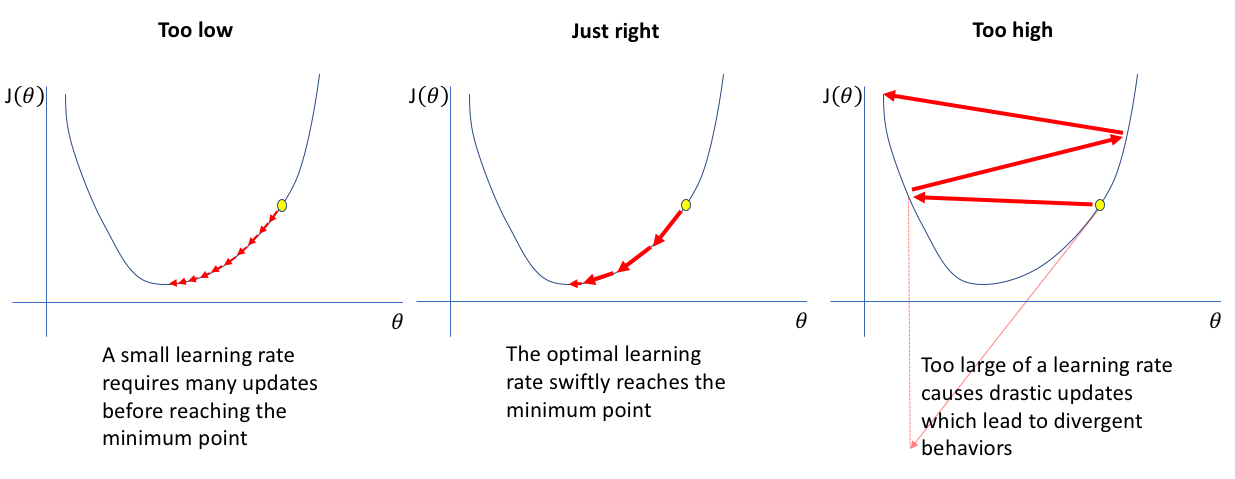
The learning rate \(\eta\) governs the amplitude of updates.

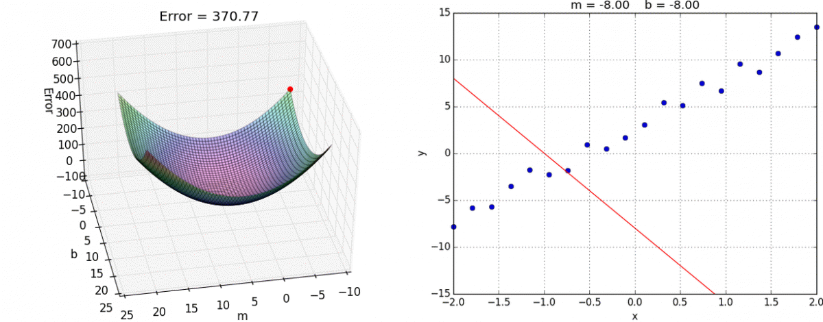
\[\pmb{\theta}_{next} = \pmb{\theta} - \eta\nabla_{\theta}\mathcal{L}(\pmb{\theta})\]

Interactive example#

Gradient descent types#

Batch: use the whole dataset to compute gradients.
- Safe but potentially slow.
Stochastic: use only one sample.
- Fast but potentially erratic.
Mini-Batch: use a small set of samples (10-1000).
- Good compromise.

Example: applying stochastic gradient descent to predict country happiness#

# Create a Linear Regression model (based on Stochastic Gradient Descent)
sgd_model_uni = SGDRegressor()

# Train and test the model on univariate data
train_model(sgd_model_uni, x_train_uni, y_train_uni)
test_model(sgd_model_uni, x_test_uni, y_test_uni)

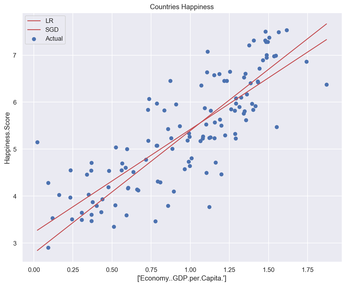
Model weights: [2.61134312], bias: [2.78170114]
Training error: 0.47787
Test error: 0.40978

# Plot data and models predictions
plot_univariate(
    x_train_uni,
    y_train_uni,
    input_features_uni,
    target_feature,
    model_list={"LR": lr_model, "SGD": sgd_model_uni},
)

../_images/75c462afb2a614161583f4a41ef325b1ee59751bb4aaffe329c7621e4727e658.png

Pros/cons of iterative approach#

Pros:

Works well with a large number of features.
MSE loss function convex => guarantee of a global minimum.

Cons:

Convergence depends on learning rate and GD type.
Dependant on feature scaling.

Polynomial Regression#

General idea#

How can a linear model fit non-linear data?
Solution: add powers of each feature as new features.
The hypothesis function is still linear.
High-degree polynomial regression can be subject to severe overfitting.

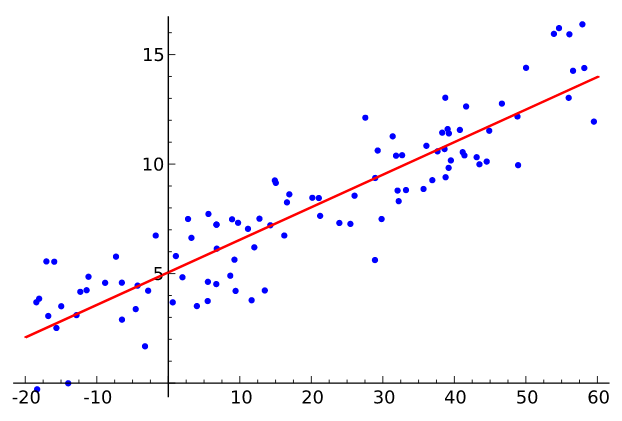
Example: fitting a quadratic curve with polynomial regression#

(Heavily inspired by Chapter 4 of Hands-On Machine Learning by Aurélien Géron)

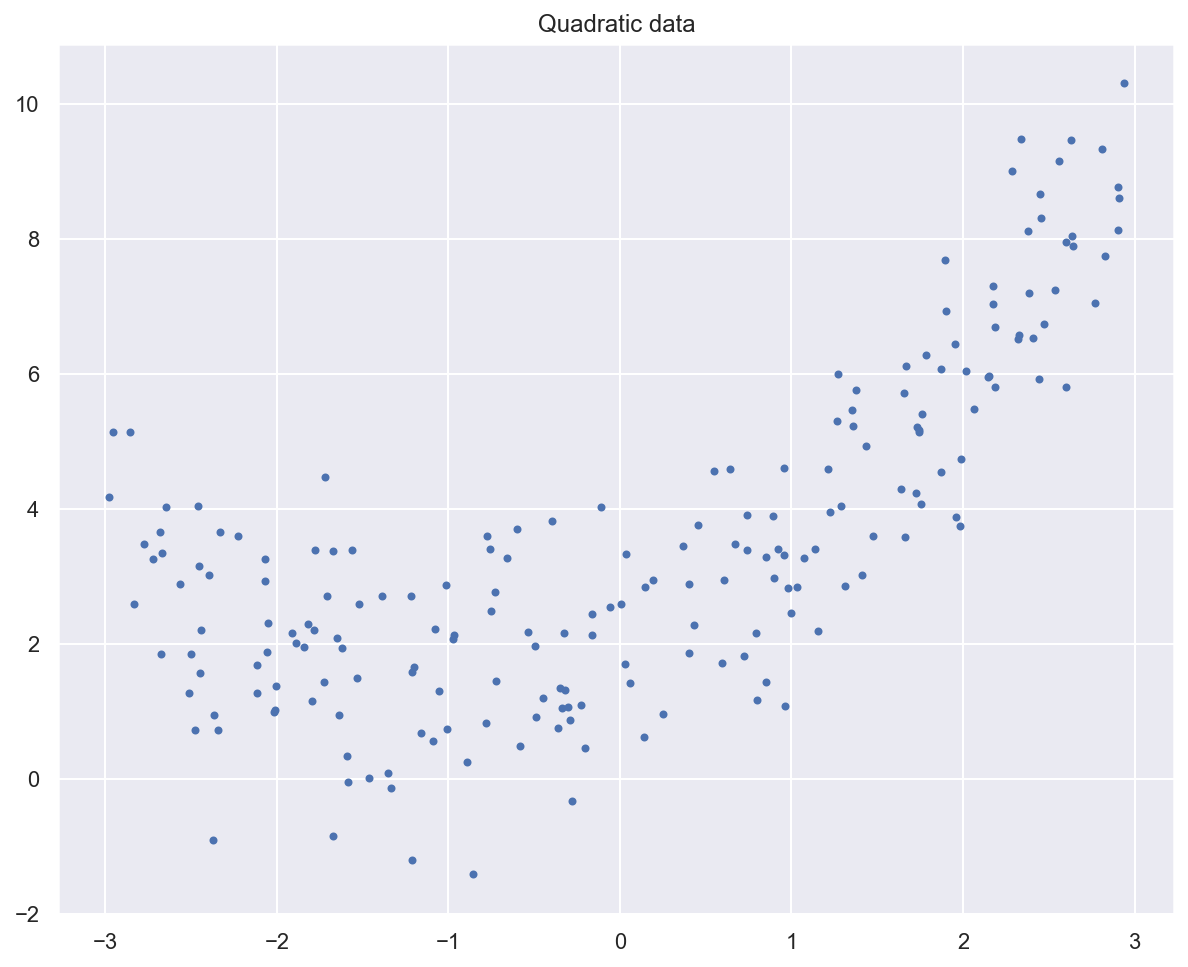
# Generate quadratic data with noise
# (ripped from https://github.com/ageron/handson-ml2)

m = 200
# Generate m data samples between -3 and 3
x_quad = 6 * np.random.rand(m, 1) - 3

# y = 0,5x^2 + x + 2 + noise
y_quad = 0.5 * x_quad**2 + x_quad + 2 + np.random.randn(m, 1)

# Plot generated data
plt.plot(x_quad, y_quad, "b.")
plt.title("Quadratic data")
plt.show()

../_images/0bbe139d1fe494fa28e5f07f95abe3cf130f1f894802f4cb66225e2a6e9476ed.png

print(f"Initial feature for first sample: {x_quad[0]}")

# Add polynomial features to the dataset
poly_degree = 2
poly_features = PolynomialFeatures(degree=poly_degree, include_bias=False)
x_quad_poly = poly_features.fit_transform(x_quad)

print(f"New features for first sample: {x_quad_poly[0]}")

Initial feature for first sample: [-1.7196066]
New features for first sample: [-1.7196066   2.95704685]

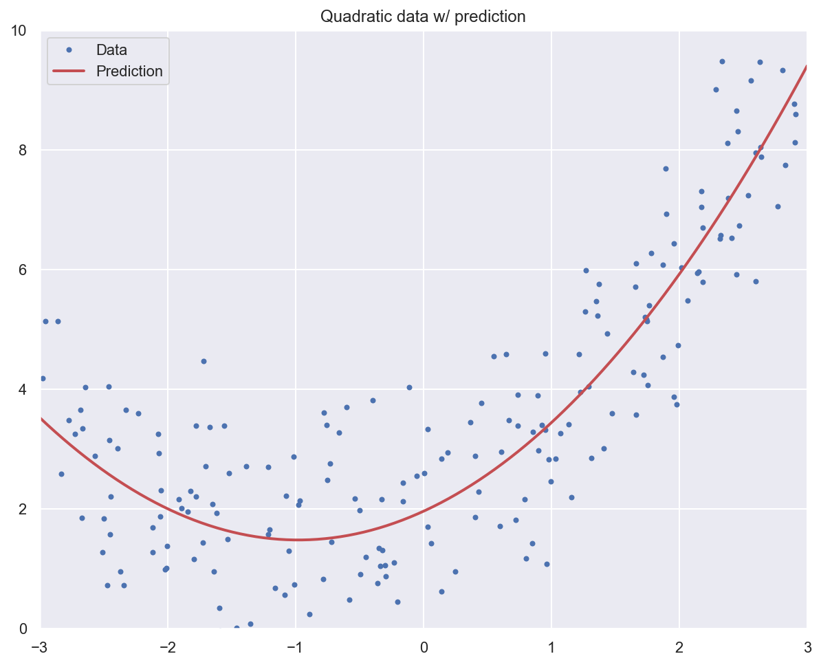
# Fit a linear regression model to the extended data
lr_model_poly = LinearRegression()
lr_model_poly.fit(x_quad_poly, y_quad)

# Should be close to [1, 0,5] and 2
print(f"Model weights: {lr_model_poly.coef_}, bias: {lr_model_poly.intercept_}")

Model weights: [[0.97997452 0.50063141]], bias: [1.9560053]

# Plot data and model prediction
plt.plot(x_quad, y_quad, "b.", label="Data")
x_pred = np.linspace(-3, 3, m).reshape(m, 1)
x_pred_poly = poly_features.transform(x_pred)
y_pred = lr_model_poly.predict(x_pred_poly)
plt.plot(x_pred, y_pred, "r-", linewidth=2, label="Prediction")
plt.axis([-3, 3, 0, 10])
plt.legend()
plt.title("Quadratic data w/ prediction")
plt.show()

../_images/dabd7294bcbac4a7de8fa50e381e3fcc7f20c72fed4b10712d442ce46221fd9b.png

Regularization#

General idea#

Solution against overfitting: constraining model parameters to take small values.
Ridge regression (using l2 norm):

\[\mathcal{L}(\pmb{\theta}) = \mathrm{MSE}(\pmb{\theta}) + \frac{\lambda}{2}\sum_{i=1}^n \theta_i^2\]

Lasso regression (using l1 norm):

\[\mathcal{L}(\pmb{\theta}) = \mathrm{MSE}(\pmb{\theta}) + \lambda\sum_{i=1}^n |\theta_i|\]

\(\lambda\) is called the regularization rate.

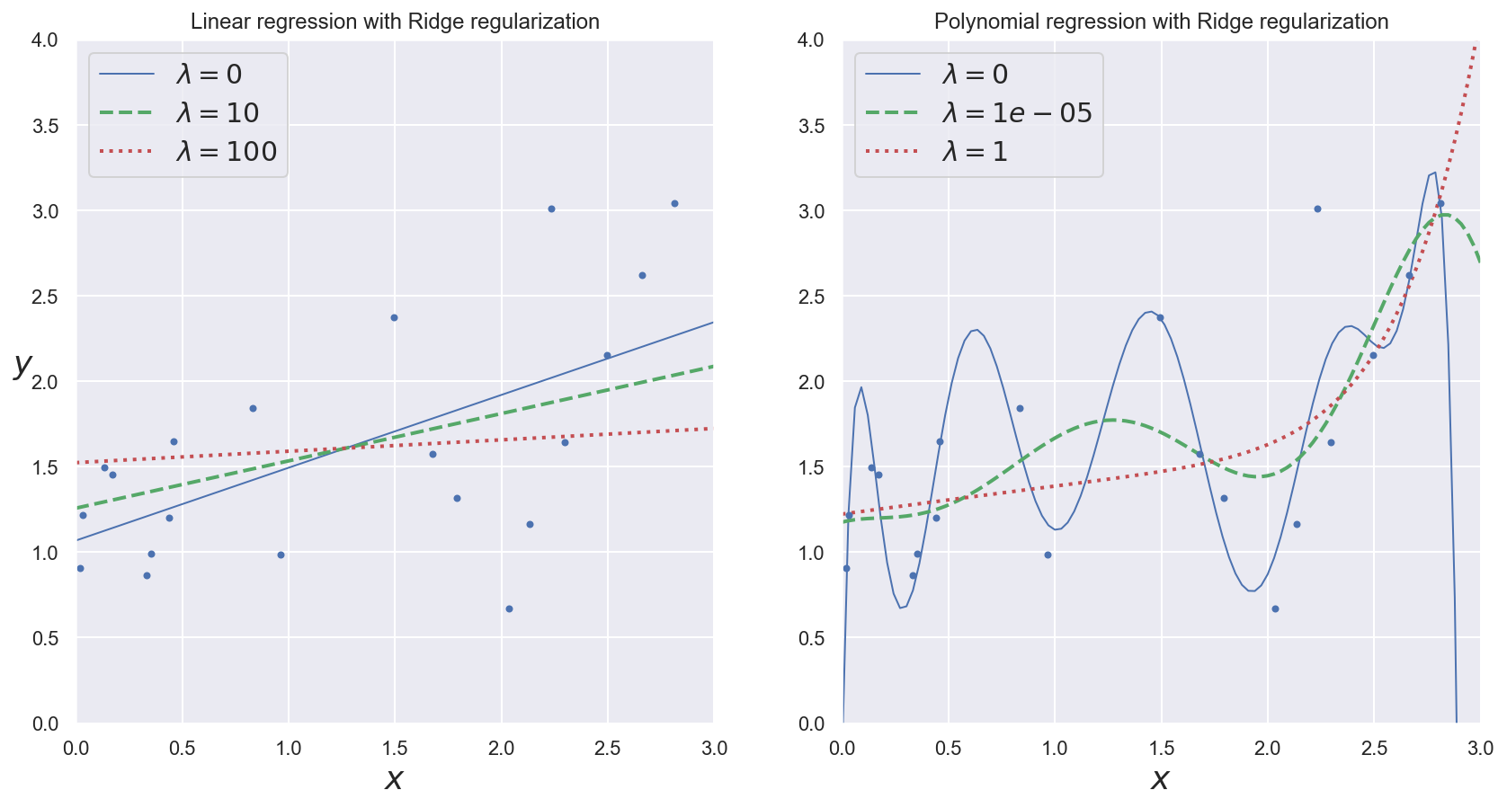
Example: observing the effects of regularization rate#

(Heavily inspired by Chapter 4 of Hands-On Machine Learning by Aurélien Géron)

m = 20
x_reg = 3 * np.random.rand(m, 1)
y_reg = 1 + 0.5 * x_reg + np.random.randn(m, 1) / 1.5
x_new = np.linspace(0, 3, 100).reshape(100, 1)

# Plot data and predictions with varying regularization rates
plt.figure(figsize=(14,7))
plt.subplot(121)
plot_model(Ridge, polynomial=False, lambdas=(0, 10, 100), random_state=42)
plt.ylabel("$y$", rotation=0, fontsize=18)
plt.title("Linear regression with Ridge regularization")
plt.subplot(122)
plot_model(Ridge, polynomial=True, lambdas=(0, 10**-5, 1), random_state=42)
plt.title("Polynomial regression with Ridge regularization")
plt.show()

../_images/535de8e4d743252af80e39ff2aae066969cd5e8ccf84ba3594af70e494a095e3.png

Linear Regression

Contents

Linear Regression#

Environment setup#

Introduction#

Linear regression in a nutshell#

Problem formulation#

Example: using a linear model to predict country happiness#

Data loading and analysis#

Univariate regression#

Example: predict country happiness using only GDP#

Data splitting#

Data plotting#

Analytical approach: normal equation#

Problem formulation#

Loss function#

Analytical solution#

Math proof (optional)#

Vectorized notation#

Vectorized loss#

Loss gradient#

Computation of loss gradient terms#

Final gradient expression#

Loss minimization#

Example: applying Normal Equation to predict country happiness#

Multivariate regression#

Pros/cons of analytical approach#

Iterative approach: gradient descent#

Method description#

Computation of gradients#

Parameters update#

Interactive example#

Gradient descent types#

Example: applying stochastic gradient descent to predict country happiness#

Pros/cons of iterative approach#

Polynomial Regression#

General idea#

Example: fitting a quadratic curve with polynomial regression#

Regularization#

General idea#

Example: observing the effects of regularization rate#