Training models

Environment setup

import platform

print(f"Python version: {platform.python_version()}")

Python version: 3.11.1

import torch

print(f"PyTorch version: {torch.__version__}")

PyTorch version: 2.0.1

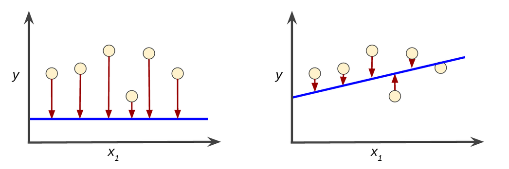
Problem formulation

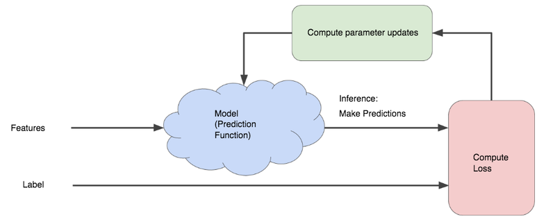
Model lifecycle

There are two (repeatable) phases:

• Training: using training input samples, the model learns to find a relationship between inputs and labels.

• Inference: the trained model is used to make predictions.

Parameters Vs hyperparameters

• \(\pmb{\theta}\) (sometime noted \(\pmb{\omega}\)): set of model’s internal parameters, updated during training.

• Many models also have user-defined properties called hyperparameters:

  • maximum depth of a decision tree;

  • number of layers of a neural network;

  • …

• Contrary to internal parameters, they are not automatically updated during training.

• The hyperparameters directly affect the model’s performance and must be tweaked during the tuning step.

Optimization algorithm

• Used during the training phase.

• Objective: find the set of model parameters \(\pmb{\theta}^{*}\) that minimizes the loss.

• For each learning type, several algorithms of various complexity exist.

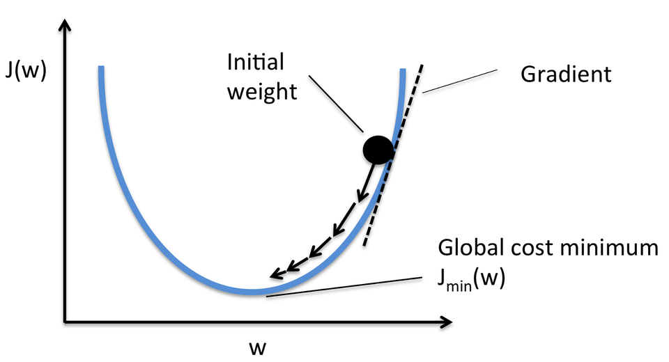
Gradient descent

An iterative approach

The model’s parameters are iteratively updated until an optimum is reached.

The gradient descent algorithm

• Used in several ML models, including neural networks.

• General idea: converging to a loss function’s minimum by updating model parameters in small steps, in the opposite direction of the loss function gradient.

The notion of gradient

• Expresses the variation of a function relative to the variation of its parameters.

• Vector containing partial derivatives of the function w.r.t. each of its \(P\) parameters.

\[\begin{split}\nabla_{\theta}\mathcal{L}(\boldsymbol{\pmb{\theta}}) = \begin{pmatrix} \ \frac{\partial}{\partial \theta_1} \mathcal{L}(\boldsymbol{\theta}) \\ \ \frac{\partial}{\partial \theta_2} \mathcal{L}(\boldsymbol{\theta}) \\ \ \vdots \\ \ \frac{\partial}{\partial \theta_P} \mathcal{L}(\boldsymbol{\theta}) \end{pmatrix}\end{split}\]

1D gradient descent (one parameter)

2D gradient (two parameters)

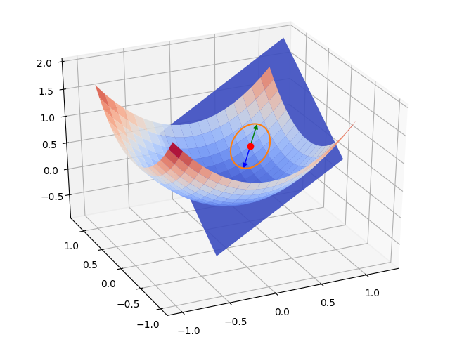
2D gradient descent

Gradient descent types

Batch Gradient Descent

The gradient is computed on the whole dataset before model parameters are updated.

• Advantages: simple and safe (always converges in the right direction).

• Drawback: can become slow and even untractable with a big dataset.

Stochastic Gradient Descent (SGD)

The gradient is computed on only one randomly chosen sample whole dataset before parameters are updated.

• Advantages:

  • Very fast.

  • Enables learning from each new sample (online learning).

• Drawback:

  • Convergence is not guaranteed.

  • No vectorization of computations.

Mini-Batch SGD

The gradient is computed on a small set of samples, called a batch, before parameters are updated.

• Combines the advantages of batch and stochastic GD.

• Default method for many ML libraries.

• The mini-batch size varies between 10 and 1000 samples, depending of the dataset size.

Model parameters update

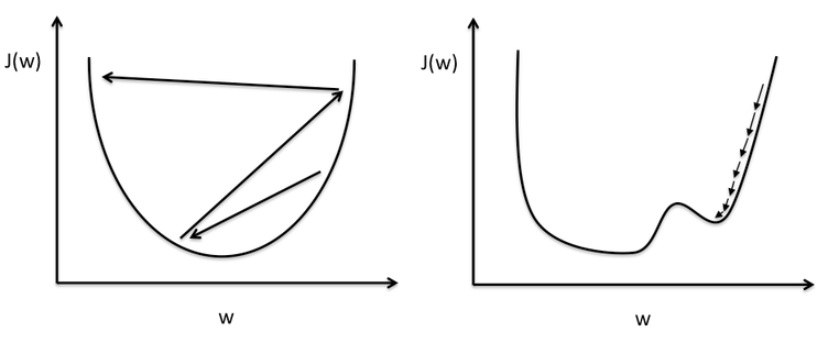
Learning rate

\(\eta\) is the update factor for parameters once gradient is computed, called the learning rate.

It has a direct impact on the “speed” of the gradient descent.

\[\pmb{\theta_{next}} = \pmb{\theta} - \eta\nabla_{\boldsymbol{\theta}}\mathcal{L}(\boldsymbol{\theta})\]

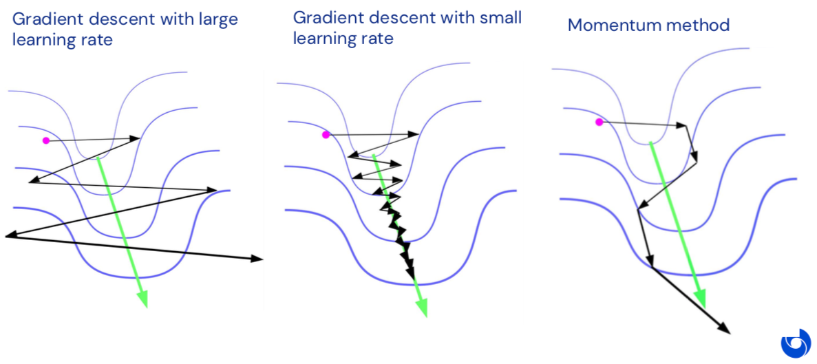
Importance of learning rate

Interactive exercise

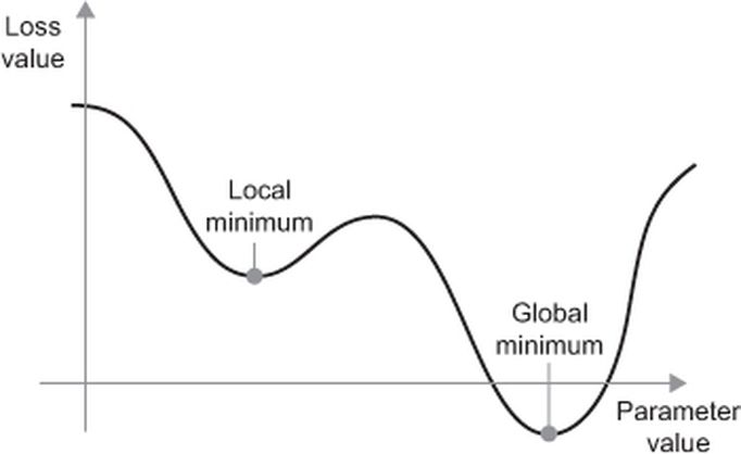
The local minima problem

Optimization algorithms

Gradient descent evolution map

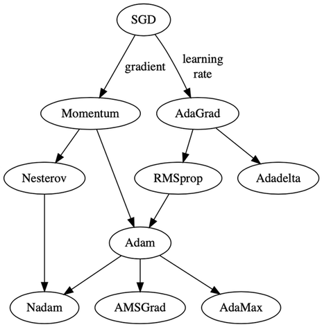
Momentum

Momentum optimization accelerates the descent speed in the direction of the minimum by accumulating previous gradients. It can also escape plateaux faster then plain GD.

Momentum equations

\[\pmb{m_{k+1}} = \beta_k \pmb{m_k} - \nabla_{\boldsymbol{\theta}}\mathcal{L}(\boldsymbol{\theta_k})\]

\[\pmb{\theta_{k+1}} = \pmb{\theta_k} + \eta_k\pmb{m_{k+1}}\]

\(\beta_k \in [0,1]\) is a friction factor that prevents gradients updates from growing too large. A typical value is 0.9.

Momentum Vs plain GD

RMSprop

RMSprop decays the learning rate differently for each parameter, scaling down the gradient vector along the steepest dimensions. The underlying idea is to adjust the descent direction a bit more towards the global minimum.

\[\pmb{v_{k+1}} = \beta_k \pmb{v_k} + (1-\beta_k) \left(\nabla_{\boldsymbol{\theta}}\mathcal{L}(\boldsymbol{\theta_k})\right)^2\]

\[\pmb{\theta_{k+1}} = \pmb{\theta_k} - \frac{\eta_k}{\sqrt{\pmb{v_{k}}+\epsilon}}\nabla_{\boldsymbol{\theta}}\mathcal{L}(\boldsymbol{\theta_k})\]

\(\epsilon\) is a smoothing term to avoid divisions by zero. A typical value is \(10^{-10}\).

Adam and other techniques

Adam (Adaptive Moment Estimation) combines the ideas of momentum and RMSprop. It is the de facto choice nowadays.

Gradient descent optimization is a rich subfield of Machine Learning. Read more in this article.

Gradients computation

Numerical differentiation

• Finite difference approximation of derivatives.

• Interpretations: instantaneous rate of change, slope of the tangent.

• Generally unstable and limited to a small set of functions.

\[g'(a) = \frac{\partial g(a)}{\partial a} = \lim_{h \to 0} \frac{g(a + h) - g(a)}{h}\]

\[\frac{\partial f(\pmb{x})}{\partial x_i} = \lim_{h \to 0} \frac{f(\pmb{x} + h\pmb{e}_i) - f(\pmb{x})}{h}\]

Symbolic differentiation

• Automatic manipulation of expressions for obtaining derivative expressions.

• Used in modern mathematical software (Mathematica, Maple…).

• Can lead to expression swell: exponentially large symbolic expressions.

\[\frac{\mathrm{d}}{\mathrm{d}x}\left(f(x)+g(x)\right) = \frac{\mathrm{d}}{\mathrm{d}x}f(x)+\frac{\mathrm{d}}{\mathrm{d}x}g(x)\]

\[\frac{\mathrm{d}}{\mathrm{d}x}\left(f(x)g(x)\right) = \left(\frac{\mathrm{d}}{\mathrm{d}x}f(x)\right)g(x)+f(x)\left(\frac{\mathrm{d}}{\mathrm{d}x}g(x)\right)\]

Automatic differentiation (autodiff)

• Family of techniques for efficiently computing derivatives of numeric functions.

• Can differentiate closed-form math expressions, but also algorithms using branching, loops or recursion.

Autodiff and its main modes

• AD combines numerical and symbolic differentiation.

• General idea: apply symbolic differentiation at the elementary operation level and keep intermediate numerical results.

• AD exists in two modes: forward and reverse. Both rely on the chain rule.

\[\frac{\mathrm{d}y}{\mathrm{d}x} = \frac{\mathrm{d}y}{\mathrm{d}w_2} \frac{\mathrm{d}w_2}{\mathrm{d}w_1} \frac{\mathrm{d}w_1}{\mathrm{d}x}\]

Forward mode autodiff

• Computes gradients w.r.t. one parameter along with the function output.

• Relies on dual numbers.

• Efficient when output dimension >> number of parameters.

Reverse mode autodiff

• Computes function output, then do a backward pass to compute gradients w.r.t. all parameters for the output.

• Efficient when number of parameters >> output dimension.

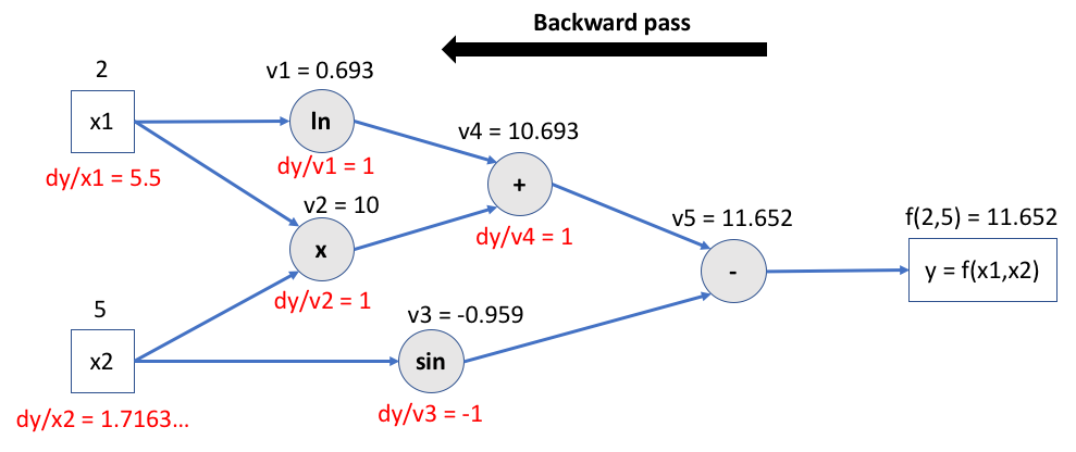
Example: reverse mode autodiff in action

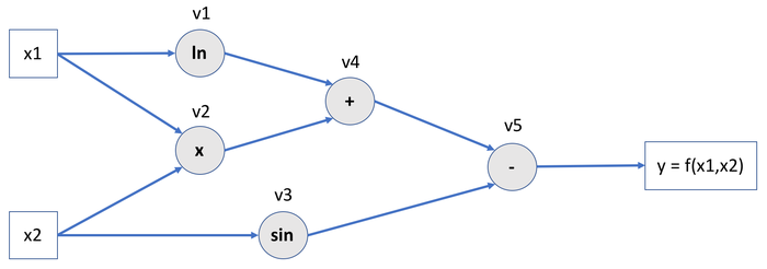
Let’s define the function \(f\) of two variables \(x_1\) and \(x_2\) like so:

\[f(x_1,x_2) = log_e(x_1) + x_1x_2 - sin(x_2)\]

It can be represented as a computational graph:

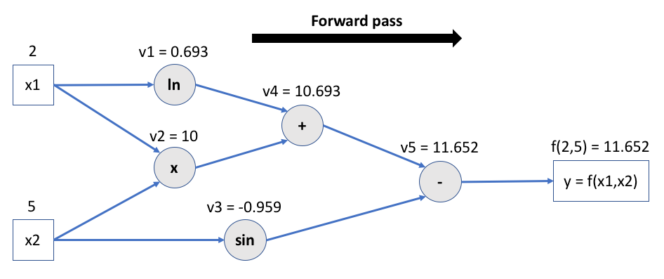
Step 1: forward pass

Intermediate values are calculated and tensor operations are memorized for future gradient computations.

Step 2: backward pass

The chain rule is applied to compute every intermediate gradient, starting from output.

\[y = f(g(x)) \;\;\;\; \frac{\partial y}{\partial x} = \frac{\partial f}{\partial g} \frac{\partial g}{\partial x}\;\;\;\; \frac{\partial y}{\partial x} = \sum_{i=1}^n \frac{\partial f}{\partial g^{(i)}} \frac{\partial g^{(i)}}{\partial x}\]

\[y=v_5=v_4-v_3\]

\[\frac{\partial y}{\partial v_4}=1\;\;\;\;\frac{\partial y}{\partial v_3}=-1\]

\[v_4=v_1+v_2\]

\[\frac{\partial y}{\partial v_1}=\frac{\partial y}{\partial v_4}\frac{\partial v_4}{\partial v_1}=1\;\;\;\;\frac{\partial y}{\partial v_2}=\frac{\partial y}{\partial v_4}\frac{\partial v_4}{\partial v_2}=1\]

\[v_1 = log_e(x_1)\;\;\;\;v_2 = x_1x_2\;\;\;\;v_3 = sin(x_2)\]

\[\frac{\partial v_1}{\partial x_1}=\frac{1}{x_1}\;\;\;\;\frac{\partial v_2}{\partial x_1}=x_2\;\;\;\;\frac{\partial v_2}{\partial x_2}=x_1\;\;\;\;\frac{\partial v_3}{\partial x_2}=cos(x_2)\]

\[\frac{\partial y}{\partial x_1}=\frac{\partial y}{\partial v_1}\frac{\partial v_1}{\partial x_1}+\frac{\partial y}{\partial v_2}\frac{\partial v_2}{\partial x_1}=\frac{1}{x_1}+x_2\]

\[\frac{\partial y}{\partial x_2}=\frac{\partial y}{\partial v_2}\frac{\partial v_2}{\partial x_2}+\frac{\partial y}{\partial v_3}\frac{\partial v_3}{\partial x_2}=x_1-cos(x_2)\]

Autodifferention with PyTorch

Autograd is the name of PyTorch’s autodifferentiation engine.

If its requires_grad attribute is set to True, PyTorch will track all operations on a tensor and provide reverse mode automatic differentiation: partial derivatives are automatically computed backward w.r.t. all involved parameters.

The gradient for a tensor will be accumulated into its .grad attribute.

More info on autodiff in PyTorch is available here.

# Create two tensors with autodiff activated
# By default, operations are not tracked on user-created tensors
x1 = torch.tensor([2.0], requires_grad=True)
x2 = torch.tensor([5.0], requires_grad=True)

# Compute f() on x1 and x2 step by step
v1 = torch.log(x1)
v2 = x1 * x2
v3 = torch.sin(x2)
v4 = v1 + v2
y = v4 - v3

print(f"v1: {v1}")
print(f"v2: {v2}")
print(f"v3: {v3}")
print(f"v4: {v4}")
print(f"y: {y}")

v1: tensor([0.6931], grad_fn=<LogBackward0>)
v2: tensor([10.], grad_fn=<MulBackward0>)
v3: tensor([-0.9589], grad_fn=<SinBackward0>)
v4: tensor([10.6931], grad_fn=<AddBackward0>)
y: tensor([11.6521], grad_fn=<SubBackward0>)

# Let the magic happen
y.backward()

print(x1.grad) # dy/dx1 = 1/2 + 5 = 5.5
print(x2.grad) # dy/dx2 = 2 - cos(5) = 1.7163...

tensor([5.5000])
tensor([1.7163])

Differentiable programming

Aka software 2.0.

“People are now building a new kind of software by assembling networks of parameterized functional blocks and by training them from examples using some form of gradient-based optimization…. It’s really very much like a regular program, except it’s parameterized, automatically differentiated, and trainable/optimizable” (Y. LeCun).