K-Nearest Neighbors

Contents

K-Nearest Neighbors#

Environment setup#

import platform

print(f"Python version: {platform.python_version()}")
assert platform.python_version_tuple() >= ("3", "6")

import numpy as np
import matplotlib.pyplot as plt
from matplotlib.colors import ListedColormap
import seaborn as sns
import pandas as pd

print(f"NumPy version: {np.__version__}")

Python version: 3.7.5
NumPy version: 1.18.1

# Setup plots
%matplotlib inline
plt.rcParams["figure.figsize"] = 10, 8
%config InlineBackend.figure_format = 'retina'
sns.set()

# Import ML packages
import sklearn

print(f"scikit-learn version: {sklearn.__version__}")

from sklearn.datasets import make_classification
from sklearn.neighbors import KNeighborsClassifier
from sklearn.model_selection import train_test_split
from sklearn.preprocessing import StandardScaler
from sklearn.metrics import plot_confusion_matrix, classification_report

scikit-learn version: 0.22.1

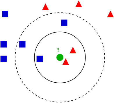
The k-nearest neighbors algorithm#

K-NN in a nutshell#

Simple, instance-based algorithm: prediction is based on the \(k\) nearest neighbors of a data sample.
No model creation, training = storing samples.

K-NN

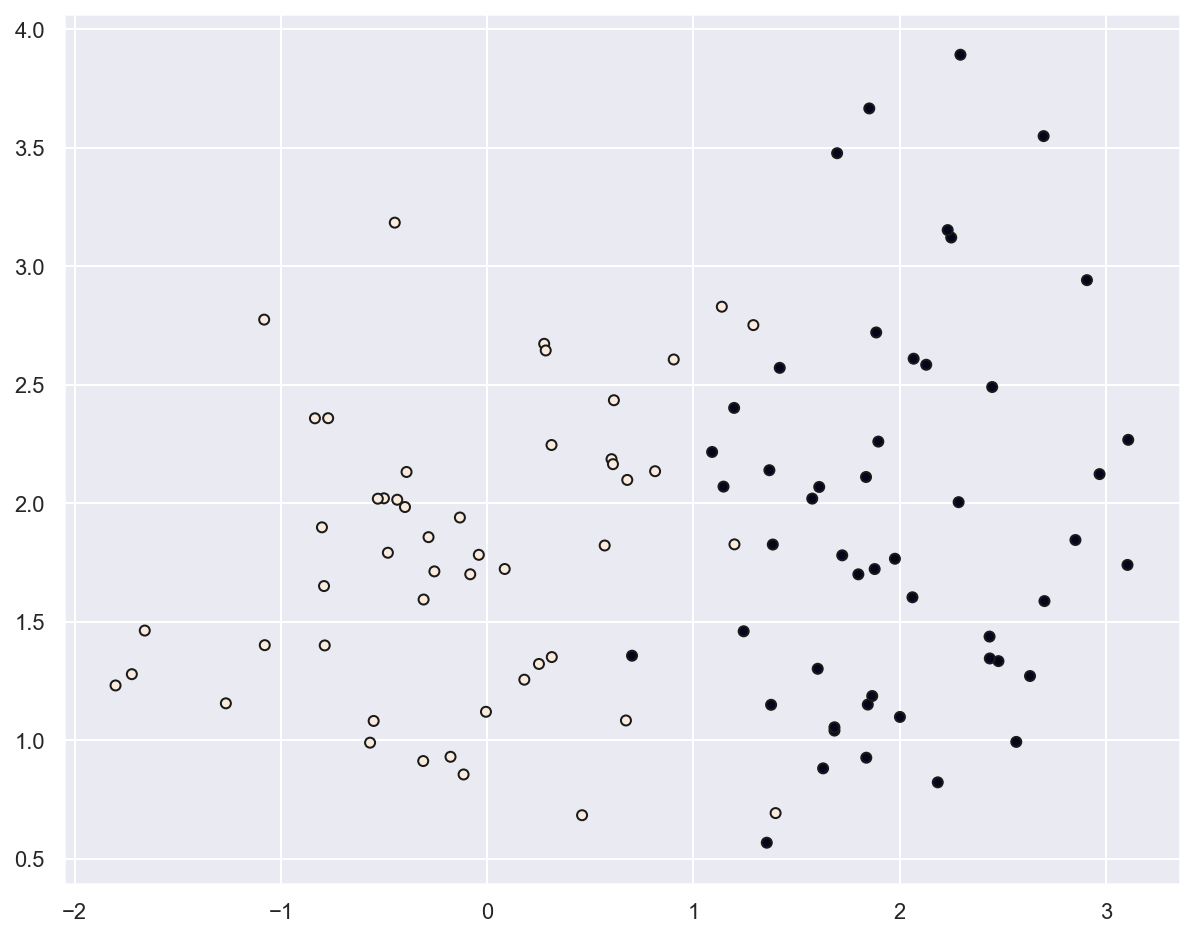
Example: planar data classification#

# Generate 2D data
x_train, y_train = make_classification(
    n_features=2, n_redundant=0, n_informative=2, random_state=1, n_clusters_per_class=1
)

rng = np.random.RandomState(2)
x_train += 2 * rng.uniform(size=x_train.shape)

print(f"x_train: {x_train.shape}. y_train: {y_train.shape}")

x_train: (100, 2). y_train: (100,)

# Plot generated data
plt.scatter(x_train[:, 0], x_train[:, 1], marker="o", c=y_train, s=25, edgecolor="k")
plt.show()

../_images/d897b2d1bd3364efddc5c8a4f519e208e4ffd451bd2cf04270204f125b7c6238.png

# Create a K-NN classifier
knn_2d_clf = KNeighborsClassifier(n_neighbors=5)
knn_2d_clf.fit(x_train, y_train)

KNeighborsClassifier(algorithm='auto', leaf_size=30, metric='minkowski',
                     metric_params=None, n_jobs=None, n_neighbors=5, p=2,
                     weights='uniform')

plot_decision_boundary(lambda x: knn_2d_clf.predict(x), x_train, y_train)

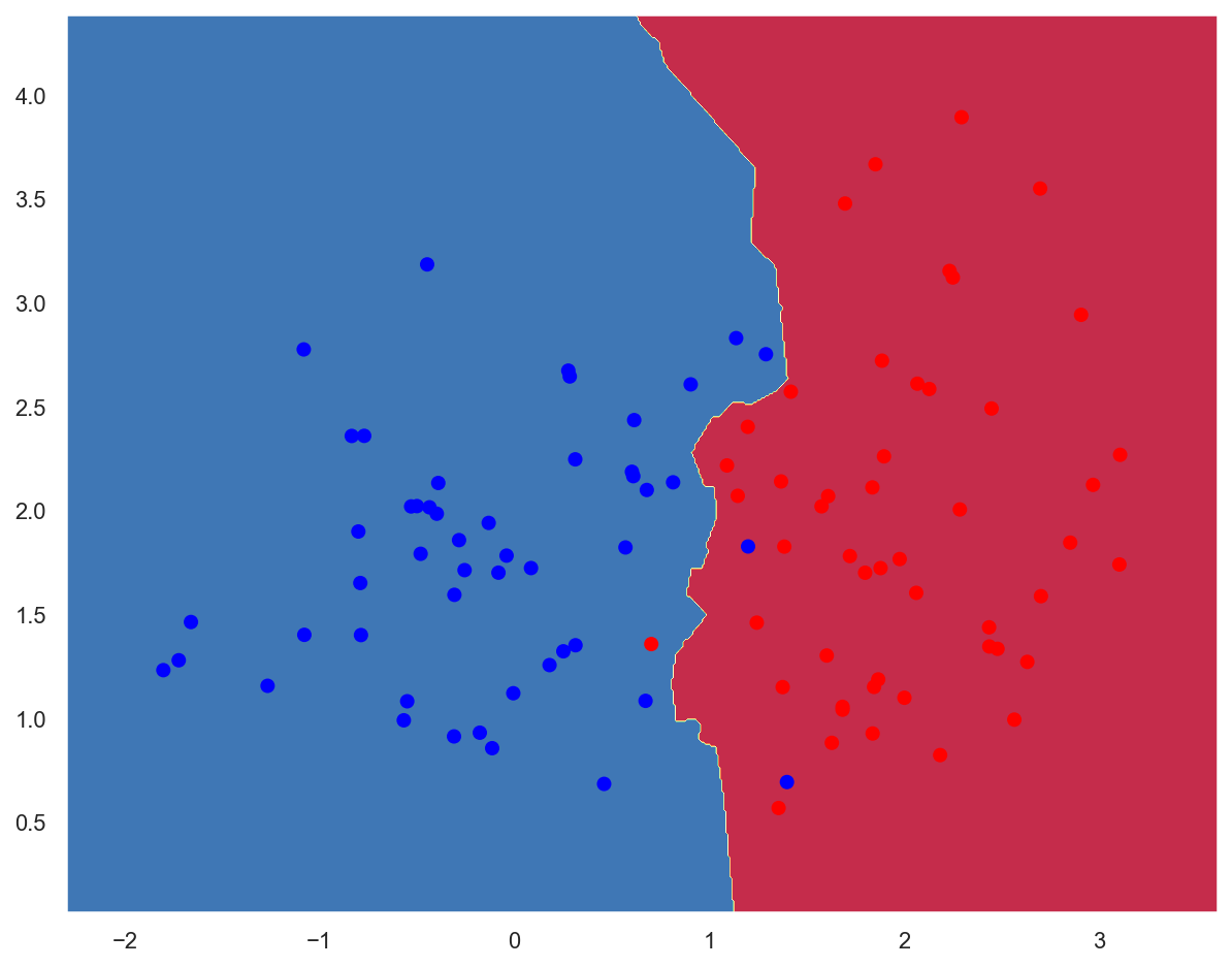
../_images/7934eae6cd27fd95a343b6614594de9e90dcd6c06718a662e7280526aa5dd6ee.png

# Evaluate  classifier
train_acc = knn_2d_clf.score(x_train, y_train)

print(f"Training accuracy: {train_acc:.05f}")

Training accuracy: 0.97000

Example: fruits classification#

Data loading#

# Download data as a text file
!wget http://www.eyrignoux.com.fr/coursIA/machineLearning/fruit_data_with_colors.txt -O fruit_data_with_colors.txt

# Load data into a DataFrame
fruits = pd.read_table("fruit_data_with_colors.txt")

# Show 10 random samples
fruits.sample(n=10)

	fruit_label	fruit_name	fruit_subtype	mass	width	height	color_score
0	1	apple	granny_smith	192	8.4	7.3	0.55
25	3	orange	spanish_jumbo	356	9.2	9.2	0.75
11	1	apple	braeburn	172	7.1	7.6	0.92
56	4	lemon	unknown	116	5.9	8.1	0.73
8	1	apple	braeburn	178	7.1	7.8	0.92
14	1	apple	golden_delicious	152	7.6	7.3	0.69
21	1	apple	cripps_pink	156	7.4	7.4	0.84
35	3	orange	turkey_navel	150	7.1	7.9	0.75
58	4	lemon	unknown	118	6.1	8.1	0.70
37	3	orange	turkey_navel	154	7.3	7.3	0.79

Data analysis#

# Evaluate class distribution
samples_count = fruits.size
for name in fruits["fruit_name"].unique():
    class_percent = fruits[fruits.fruit_name == name].size / samples_count
    print(f"{name}s : {class_percent * 100:.1f}%")

apples : 32.2%
mandarins : 8.5%
oranges : 32.2%
lemons : 27.1%

# For this scenario, we use only the mass, width, and height features of each fruit instance
x = fruits[["mass", "width", "height"]]
# Objective is to predict the fruit class
y = fruits["fruit_label"]

print(f"x: {x.shape}. y: {y.shape}")

x: (59, 3). y: (59,)

Data preprocessing#

# Split data between training and test sets with a 80/20 ratio
x_train, x_test, y_train, y_test = train_test_split(x, y, test_size=0.2)

print(f"x_train: {x_train.shape}. y_train: {y_train.shape}")
print(f"x_test: {x_test.shape}. y_test: {y_test.shape}")

x_train: (47, 3). y_train: (47,)
x_test: (12, 3). y_test: (12,)

# Standardize data
scaler = StandardScaler().fit(x_train)

x_train = scaler.transform(x_train)
x_test = scaler.transform(x_test)

Classifier creation and “training”#

# k = 5
knn_fruits_clf = KNeighborsClassifier(n_neighbors=5)
knn_fruits_clf.fit(x_train, y_train)

KNeighborsClassifier(algorithm='auto', leaf_size=30, metric='minkowski',
                     metric_params=None, n_jobs=None, n_neighbors=5, p=2,
                     weights='uniform')

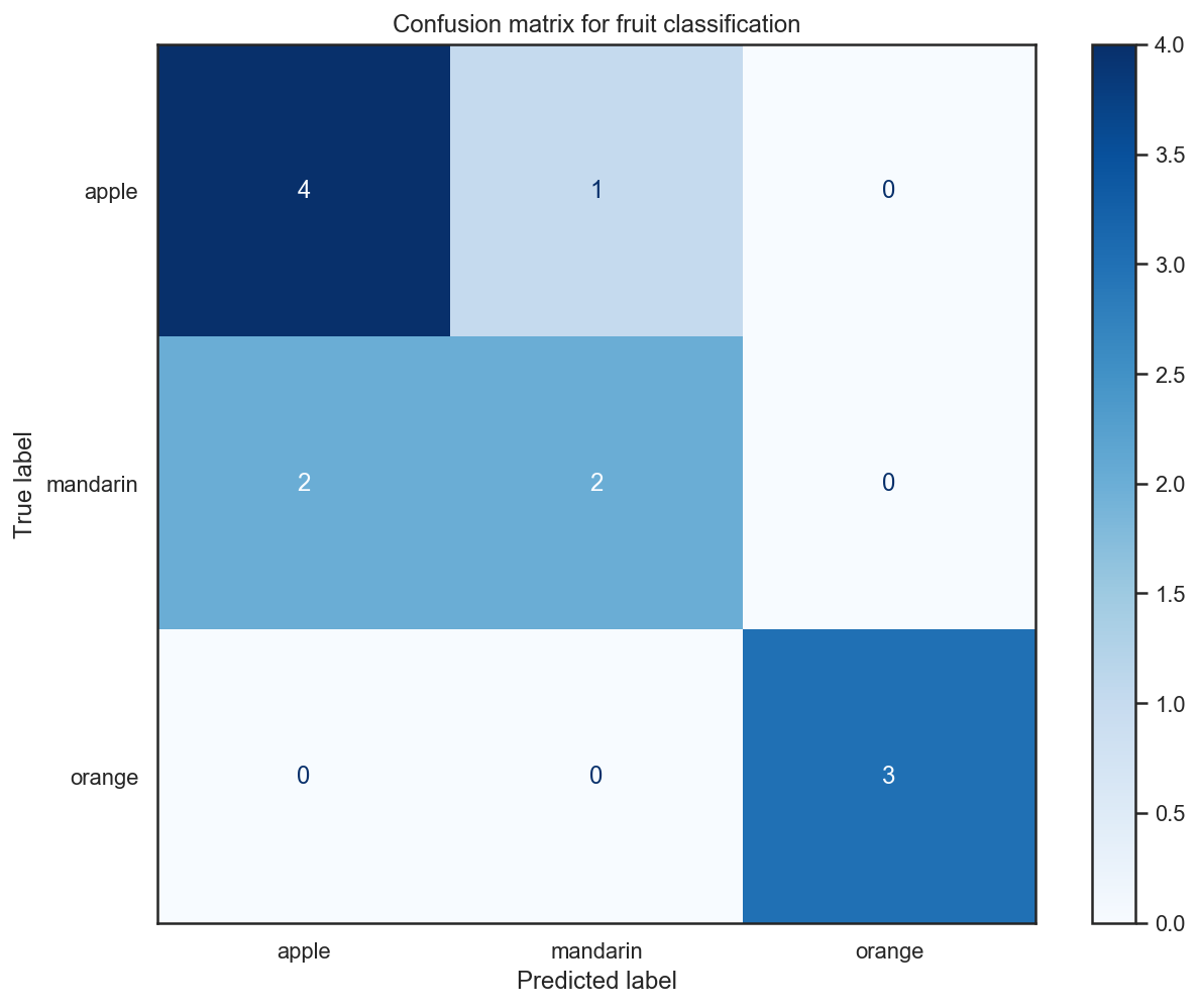
Classifier evaluation#

# Compute accuracy on training and test sets
train_acc = knn_fruits_clf.score(x_train, y_train)
test_acc = knn_fruits_clf.score(x_test, y_test)

print(f"Training accuracy: {train_acc:.05f}")
print(f"Test accuracy: {test_acc:.05f}")

Training accuracy: 0.89362
Test accuracy: 0.75000

# Plot the confusion matrix for test data
with sns.axes_style("white"):  # Temporary hide Seaborn grid lines
    display = plot_confusion_matrix(
        knn_fruits_clf,
        x_test,
        y_test,
        display_labels=fruits["fruit_name"].unique(),
        cmap=plt.cm.Blues,
    )
    display.ax_.set_title("Confusion matrix for fruit classification")
    plt.show()

../_images/85143e68f3a6ea021517d3828f183e5d6044d0936afb3a54b44ea78919520b07.png

# Compute classification metrics
print(classification_report(y_test, knn_fruits_clf.predict(x_test)))

              precision    recall  f1-score   support

           1       0.67      0.80      0.73         5
           3       0.67      0.50      0.57         4
           4       1.00      1.00      1.00         3

    accuracy                           0.75        12
   macro avg       0.78      0.77      0.77        12
weighted avg       0.75      0.75      0.74        12

Using the classifier for predictions#

# create a mapping from fruit label value to fruit name to make results easier to interpret
lookup_fruit_name = dict(zip(fruits.fruit_label.unique(), fruits.fruit_name.unique()))

# first example: a small fruit with mass 20g, width 4.3 cm, height 5.5 cm
fruit_prediction = knn_fruits_clf.predict([[20, 4.3, 5.5]])
lookup_fruit_name[fruit_prediction[0]]

'orange'

# second example: a larger, elongated fruit with mass 100g, width 6.3 cm, height 8.5 cm
fruit_prediction = knn_fruits_clf.predict([[100, 6.3, 8.5]])
lookup_fruit_name[fruit_prediction[0]]

'orange'

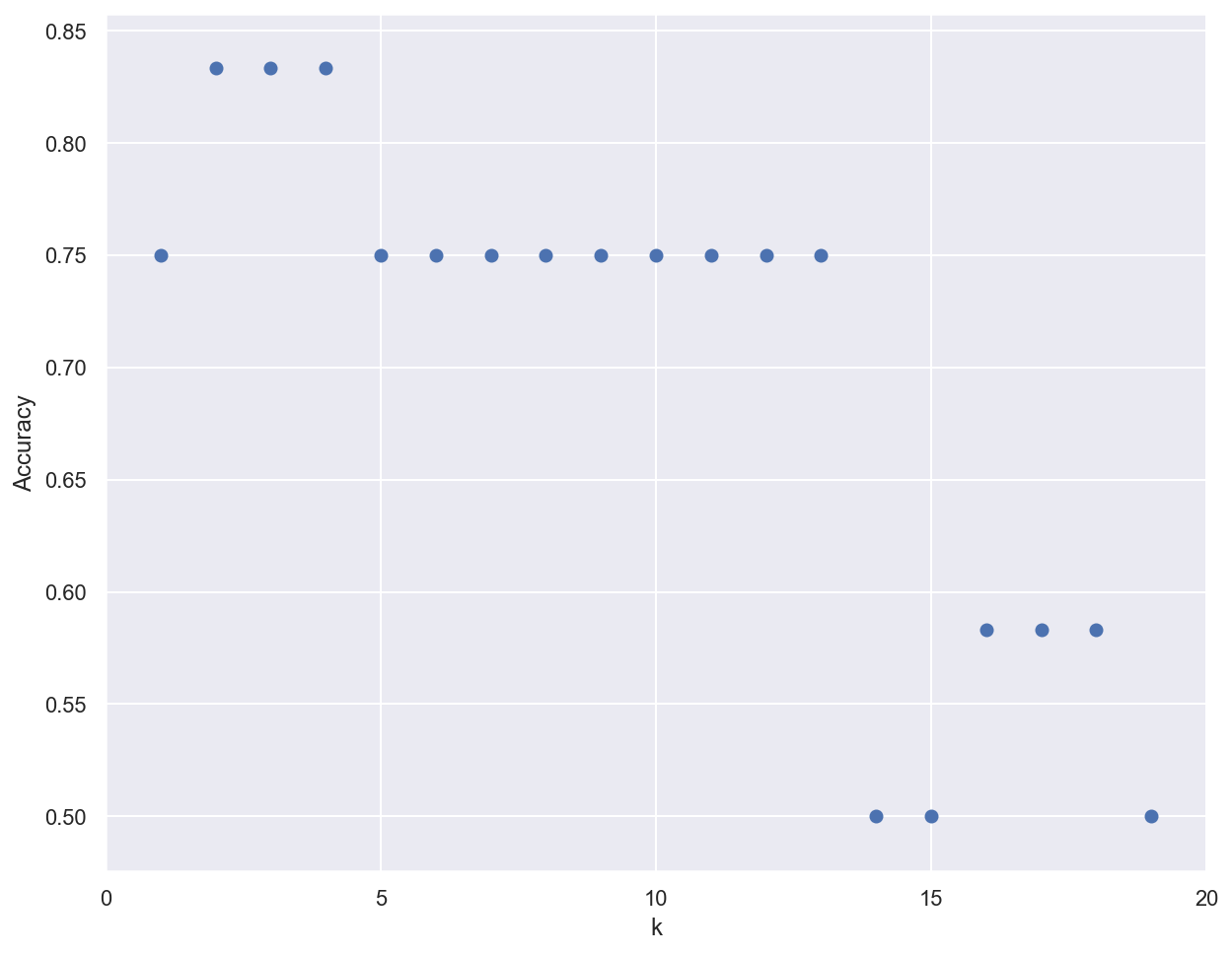
Importance of the `k` parameter#

k_range = range(1, 20)
scores = []

# Train several classifiers with different values for k
for k in k_range:
    knn_clf = KNeighborsClassifier(n_neighbors=k)
    knn_clf.fit(x_train, y_train)
    scores.append(knn_clf.score(x_test, y_test))

# Plot results
plt.figure()
plt.xlabel('k')
plt.ylabel('Accuracy')
plt.scatter(k_range, scores)
plt.xticks([0,5,10,15,20]);

../_images/5f48f5c27d4bb50266461369931e70df3f183e4e272b5e965222451a92da4661.png

TODO

Planar data: add multiclass data
Better looking graphs: https://stackabuse.com/k-nearest-neighbors-algorithm-in-python-and-scikit-learn/